[계산사진학] Image Warping 1

JAEYOON SIM·2021년 11월 15일

Computational Photography

목록 보기

20/34

Image processing에는 주로 다루는 2개의 image operation이 있다. 그 중 하나는 filtering이고, 나머지 하나는 warping이다.
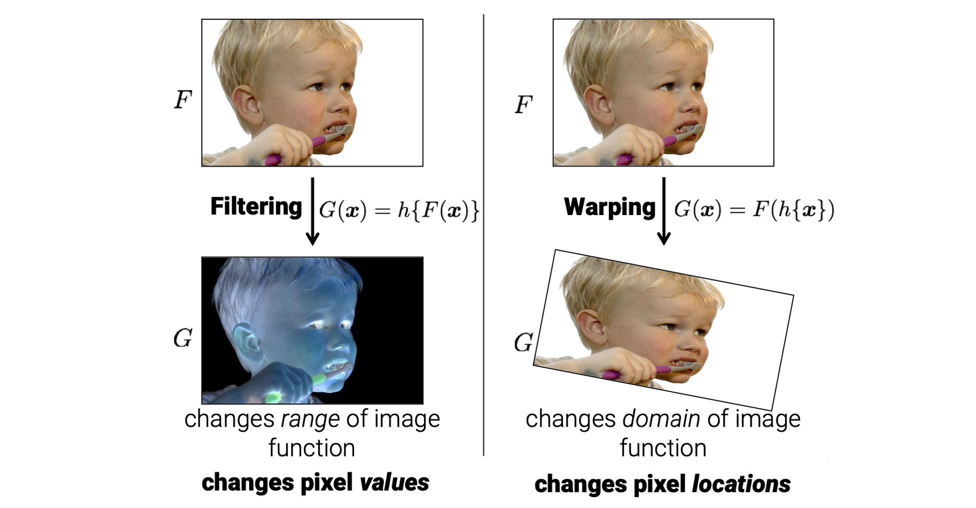Filtering은 pixel의 값을 바꾸는 것이지만, warping은 pixel의 위치를 바꾸는 것이다. 우리는 수학적으로 위와 같이 filtering과 warping을 표현할 수 있다. Filtering은 수학적으로 image function의 범위를 바꾸지만, warping은 수학적으로 image function의 domain을 바꿔준다. 이번에는 둘 중에서 warping에 대해서 이야기해보려고 한다.

Image warping의 pseudocode는 다음과 같다.
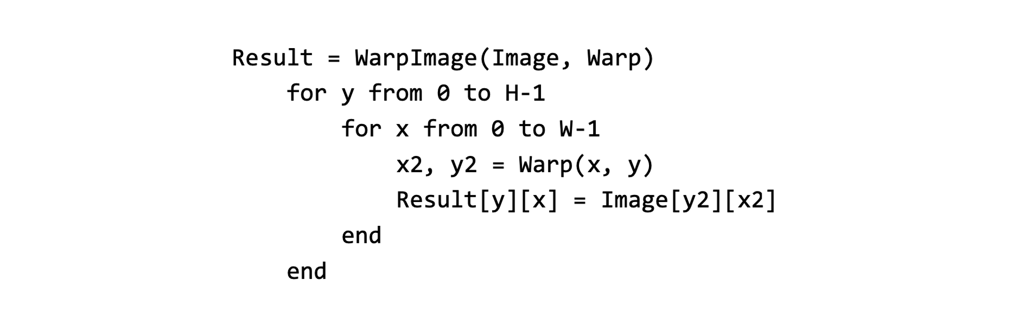여기서 우리는 WarpImage라는 function을 부르고, 2개의 parameter를 input으로 가지게 된다. 첫번째 parameter는 source image이고, 두번째 parameter는 얼마나 pixel의 위치가 바뀌는지 정해주는 warping function이다. 이 function은 반복문 내에서 모든 pixel에 대해서 동작하게 된다. 각각의 pixel에서 이에 대응되는 source pixel의 위치를 계산하고, function은 sourc pixel의 위치로부터 pixel 값을 현재 target으로 하는 pixel의 위치에 복사한다. 이 과정은 매우 간단하다.

Parametric Global Warping

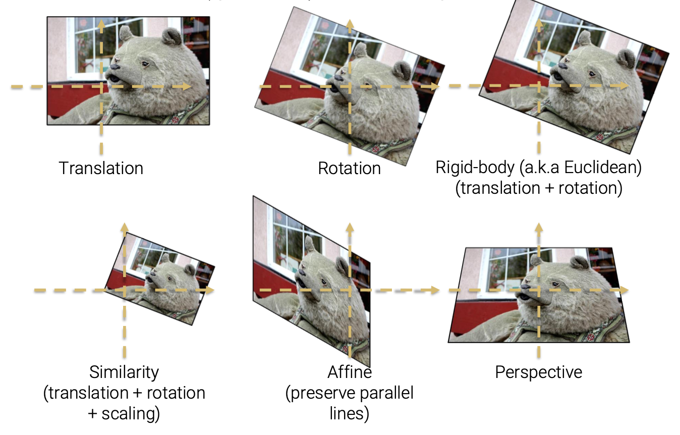
이제 위에서 본 warping function에 대해서 좀 더 자세하게 볼 것이다. 많은 warping 방법들 중에서 우리가 이번에 다룰 것은 parametrice global warping이다. 다음은 6가지 다른 warping operation들이다.
이 operation들은 가장 근본이 되는 parametric global warping operation들이다.

Translation은 image를 x축과 y축을 따라서 shifting해준다. Rotation은 image를 원점을 기준으로 회전시켜준다. Rigid-body transformation은 Euclidean transformation으로도 잘 알려져 있으며, 이는 translation과 rotation을 조합한 것이다. Similarity transformation은 translation과 rotation 외에도 scaling을 조합한 것이다. 이는 rigid-body transformation에다가 scaling을 더한 것으로 볼 수 있다. Affine transformation은 parallel line들을 보존하는 2D transformation으로, 이는 similarity transformation의 superset이다. 마지막으로 perspective transformation은 parallel line들을 보존하지 못하는, 더 일반적인 transformation이다. Affine과 perspective transformation은 나중에 더 자세하게 다룰 것이다.

Parametric global warping은 pixel의 좌표를 바꾸는 transformation이다.
좌측이 source pixel $p$ 이고, 우측이 target pixel $p'$ 이다. 그리고 이를 바꿔주는 transformation function은 $T$ 이다. 그래서 T는 다음과 같이 좌표를 바꿔준다.

p' = T(p)

Parametric global warping에서 global이라는 단어는 동일한 $T$ 가 모든 pixel에 적용한다는 것이고, parametric이라는 단어는 몇개 안되는 parameter들에 의해서 $T$ 가 설명될 수 있다는 것이다. 예를 들어서, 다음은 rotaion이다.
Rotation이 parametric global warping인 이유는 우리가 모든 pixel에 동일한 rotation matrix를 적용하면서, 이 matrix가 오직 parameter $\theta$ 하나만으로도 설명될 수 있기 때문이다.

Scaling

이제 간단한 warping 예시들을 볼 것이다. 첫번째는 image scaling이다. Scaling은 다음과 같이 image를 키우거나 줄이는 역할을 한다.
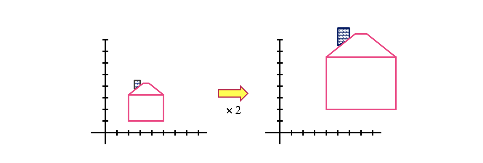좌표를 scaling한다는 것은 어떠한 scalar에 의해서 각각의 성분들이 곱해지는 것을 의미한다. Uniform scaling은 모든 성분들에 대해서 이 scalar 값이 같은 것을 의미한다. 그리고 non-uniform scaling도 있다.
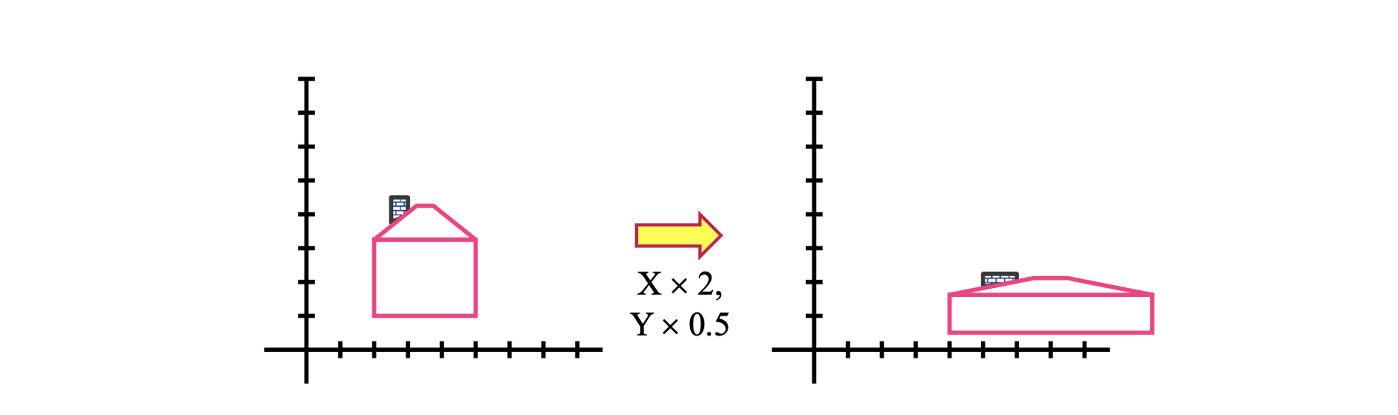Non-uniform scaling은 각각의 성분에 대해서 서로 다른 scalar를 사용하는 것을 의미한다. 그래서 우리는 위와 같이 종횡비를 바꿔서 image에 적용할 수 있다.

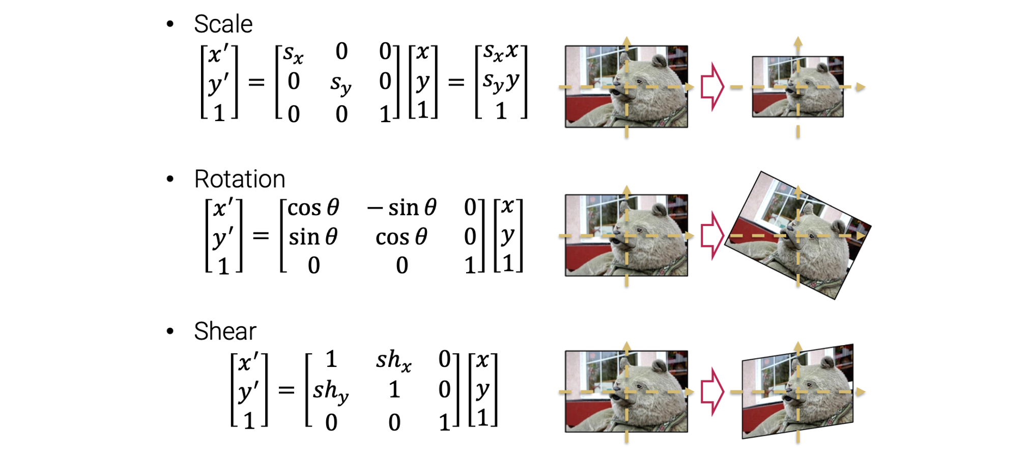
Scaling operation은 다음과 같이 2개의 간단한 식을 사용해서 나타낼 수 있다.
$\text{Scaling operation:}$

x' = ax

y' = by

$x, y$ 는 각각 source pixel의 $x$ 좌표와 $y$ 좌표를 의미하고, $a, b$ 는 각각의 component들에 대한 scaling factor이다. 그리고 $x', y'$ 은 warped 좌표를 의미한다. 우리는 이러한 식들을 다음과 같이 matrix form으로 다시 나타낼 수 있다.

$\text{In matrix form:}$

\begin{bmatrix} x' \\ y' \end{bmatrix} = \begin{bmatrix} a & 0 \\ 0 & b \end{bmatrix} \begin{bmatrix} x \\ y \end{bmatrix}

그리고 scaling의 inverse는 또한 다시 scaling이 되고, 다음과 같이 나타낼 수 있다.

$\text{Iverse is also scaling:}$

\begin{bmatrix} x' \\ y' \end{bmatrix} = \begin{bmatrix} 1/a & 0 \\ 0 & 1/b \end{bmatrix} \begin{bmatrix} x \\ y \end{bmatrix}

2D Rotation

또 다른 간단한 warping operation으로는 2D roation이 있고, 다음과 같이 matrix form으로 나타낼 수 있다.

$\text{Roation operation (in matrix form):}$

\begin{bmatrix} x' \\ y' \end{bmatrix} = \underbrace{ \begin{bmatrix} cos\theta & -sin\theta \\ sin\theta & cos\theta \end{bmatrix}}_{R} \begin{bmatrix} x \\ y \end{bmatrix}

간단하게 $2\times2$ matrix로 표현했다. 그리고 우리는 이미 rotation의 inverse는 다시 roation이라는 사실을 알고있다. 좀 더 자세하세 $\theta$ 에 의한 rotation의 inverse는 $-\theta$ 에 의한 rotation이 된다. 그래서 inverse는 transpose와 똑같아지게 된다.

$\text{Inverse (rotation by }-\theta\text{):}$

\begin{bmatrix} x' \\ y' \end{bmatrix} = \begin{bmatrix} cos(-\theta) & -sin(-\theta) \\ sin(-\theta) & cos(-\theta) \end{bmatrix} \begin{bmatrix} x \\ y \end{bmatrix}

\iff

\begin{bmatrix} x' \\ y' \end{bmatrix} = \begin{bmatrix} cos\theta & sin\theta \\ -sin\theta & cos\theta \end{bmatrix} \begin{bmatrix} x \\ y \end{bmatrix}

R^{-1}=R^T

Shearing

Shearing operation은 다음과 같이 object의 모양을 skew, 즉 비스듬하게 하는 것이다.
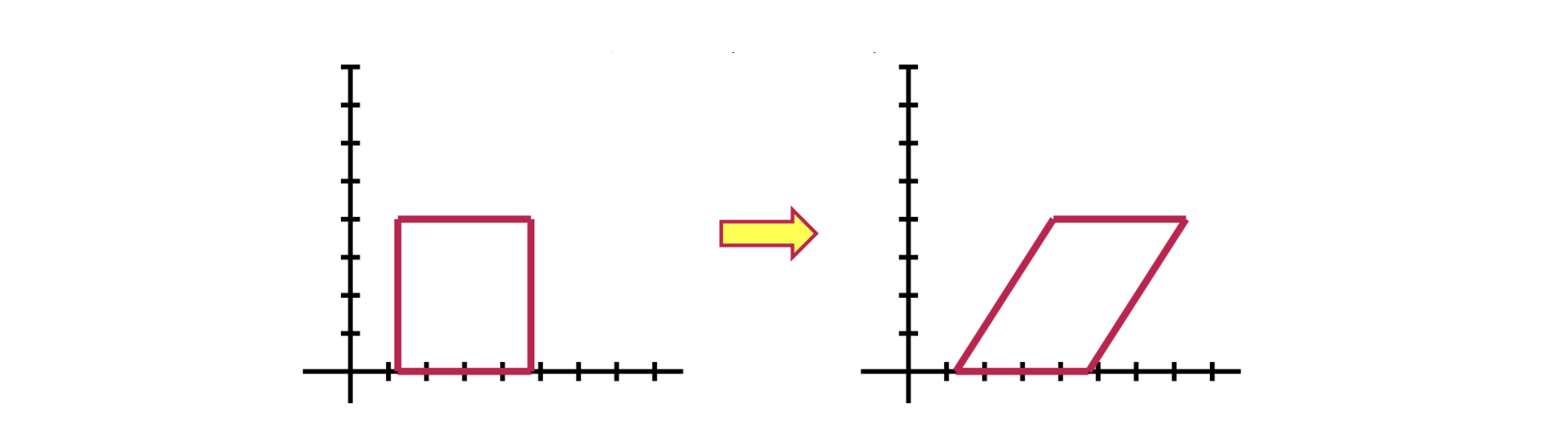Shearing은 x축이나 y축을 따라 각각 비례해서 image를 바꿔준다. 그래서 shearing operation은 다음과 같이 2개의 간단한 식을 통해서 나타낼 수 있고, 이는 또한 matrix form으로 바꿔서 표현할 수 있다.

$\text{Shearing operation:}$

x' = x + sh_x \ast y

y' = sh_y \ast x + y

$\text{In matrix form:}$

\begin{bmatrix} x' \\ y' \end{bmatrix} = \begin{bmatrix} 1 & sh_x \\ sh_y & 1 \end{bmatrix} \begin{bmatrix} x \\ y \end{bmatrix}

2 x 2 Matrices

위와 같이 scaling, rotation, shearing 등과 같은 간단한 warping operation들은 간단하게 $2\times 2$ matrix를 이용해서 나타낼 수 있다. 그렇다면 어떠한 종류의 transformation이 $2\times 2$ matrix로 나타낼 수 있는 것일까? 2D identity는 어떠한가?

$\text{2D identity:}$

x'=x

y'=y

\begin{bmatrix} x' \\ y' \end{bmatrix} = \begin{bmatrix} 1 & 0 \\ 0 & 1 \end{bmatrix} \begin{bmatrix} x \\ y \end{bmatrix}

2D identity도 위와 같이 matrix form으로 나타낼 수 있다. 그렇다면 원점으로부터 2D scaling은 어떠한가?

$\text{2D scale around (0,0):}$

x'=S_x \ast x

y'=S_y \ast y

\begin{bmatrix} x' \\ y' \end{bmatrix} = \begin{bmatrix} S_x & 0 \\ 0 & S_y \end{bmatrix} \begin{bmatrix} x \\ y \end{bmatrix}

이 역시 이미 봤었기에 당연하게 $2\times 2$ matrix로 나타낼 수 있다. 이번에는 원점으로부터 2D rotation을 어떠할까?

$\text{2D rotation around (0,0):}$

x'=cos\Theta \ast x - sin\Theta \ast y

y'=sin\Theta \ast x + cos\Theta \ast y

\begin{bmatrix} x' \\ y' \end{bmatrix} = \begin{bmatrix} cos\Theta & -sin\Theta \\ sin\Theta & cos\Theta \end{bmatrix} \begin{bmatrix} x \\ y \end{bmatrix}

이것도 역시 가능하다. 2D shearing은 이미 보았다시피 가능하다.

$\text{2D shear:}$

x' = x + sh_x \ast y

y' = sh_y \ast x + y

\begin{bmatrix} x' \\ y' \end{bmatrix} = \begin{bmatrix} 1 & sh_x \\ sh_y & 1 \end{bmatrix} \begin{bmatrix} x \\ y \end{bmatrix}

이번에는 하나의 축과 원점을 선택해서 2D mirroring operation을 해보려고 한다.

$\text{2D mirror about Y axis:}$

x' = -x

y' = y

\begin{bmatrix} x' \\ y' \end{bmatrix} = \begin{bmatrix} -1 & 0 \\ 0 & 1 \end{bmatrix} \begin{bmatrix} x \\ y \end{bmatrix}

$\text{2D mirror over (0,0):}$

x' = -x

y' = -y

\begin{bmatrix} x' \\ y' \end{bmatrix} = \begin{bmatrix} -1 & 0 \\ 0 & -1 \end{bmatrix} \begin{bmatrix} x \\ y \end{bmatrix}

위와 같이 matrix로 가능하다. 그래서 기본적으로 많고 간단한 image warping operation들이 하나의 $2\times 2$ matrix를 사용해서 나타내는 것이 가능하다. 그렇다면 2D translation은 어떠할까? 우선, 2D translation을 다음과 같이 2개의 식으로 간단하게 나타낼 수 있다.

$\text{2D translation:}$

x' = x + t_x

y' = y + t_y

그러나 아쉽게도 이 식들을 하나의 $2\times 2$ matrix로 나타내는 것은 불가능하다. 바로 식들에 더해져 있는 constant 때문이다. Vector space에서 정의된 linear transformation은 matrix multiplication을 이용해서 나타낼 수 있다. 그래서 기본적으로 오로지 linear 2D transformation만이 $2\times 2$ matrix에 의해서 표현이 가능한 것이다. 그리고 translation은 linear 2D transformation이 아니다. 그래서 이는 $2\times 2$ matrix로 표현할 수 없는 것이다.

All 2D Linear Transformations

그렇다면 linear transformation이라는 것은 무엇일까? Image warping에서 linear transformation은 scaling, rotation, shearing, mirroring의 조합이 된다.
각각은 모두 $2\times 2$ matrix로 나타내는 것이 가능하다. 이러한 linear transformation은 몇가지 성질을 가지게 된다.

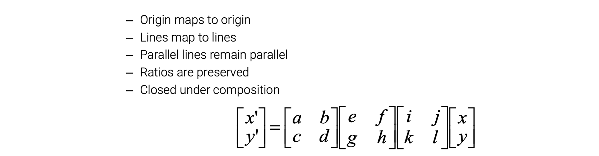원점은 원점을 mapping하고, line은 line에 mapping한다. 그리고 parallel과 ratio는 보존하고, 마지막으로 composition에는 close 되어 있다. 이는 linear transformation의 조합은 여전히 linear transformation이라는 것을 의미하고, 여러개의 $2\times 2$ matrix들로 표현하게 된다.

Compositing Transformations

Linear transformation의 경우들 중에서 우리는 단순히 여러개의 $2\times 2$ matrix를 stacking하여 다른 transformation을 구성할 수 있으며, 그 결과는 다시 하나의 $2\times 2$ matrix로 나타낼 수 있다. 예를 들어서 우리는 rotation과 scaling, 그리고 다시 rotation을 하고 싶다고 해보자.

$\text{Rotation by }\phi\text{ - scaling - rotation by }\theta\text{:}$

\begin{bmatrix} cos\theta & -sin\theta \\ sin\theta & cos\theta \end{bmatrix} \begin{bmatrix} a & 0 \\ 0 & b \end{bmatrix} \begin{bmatrix} cos\phi & -sin\phi \\ sin\phi & cos\phi \end{bmatrix} \begin{bmatrix} x \\ y \end{bmatrix} = M \begin{bmatrix} x \\ y \end{bmatrix}

각각의 operation을 연달아 적용하게 되면 이 모든 것을 똑같이 적용하는 하나의 $2\times 2$ matrix $M$ 을 얻을 수 있다. 그러나, 만약 우리가 translation을 포함하기를 원한다면, composition은 약간 복잡해지게 된다. 예를 들어 rotation을 하고 translation을 한 뒤에 scaling을 해본다해 해보자.

$\text{Rotation by }\phi\text{ - translation - scaling:}$

\begin{bmatrix} a & 0 \\ 0 & b \end{bmatrix} \Bigg(\begin{bmatrix} cos\phi & -sin\phi \\ sin\phi & cos\phi \end{bmatrix} \begin{bmatrix} x \\ y \end{bmatrix} + \begin{bmatrix} t_x \\ t_y \end{bmatrix}\Bigg)

위의 composition을 하나의 $2\times 2$ matrix로 나타내는 것은 불가능하다. Computer vision과 graphics에서 translation을 포함해서 여러개의 warping operation들을 종종 사용해야 한다. 그렇기 때문에 이러한 문제는 정말로 복잡해지게 된다.

Homogeneous Coordinates

그래서 이를 해결하고자 우리는 homogeneous 좌표계를 사용하게 된다. 이 시스템은 2차원의 좌표 정보를 3차원의 vector로 표현한다.

\underbrace{ \begin{bmatrix} x \\ y \\ z \end{bmatrix}}_\text{Homogeneous coordinates} \iff \underbrace{ \begin{bmatrix} x/w \\ y/w \end{bmatrix}}_\text{Cartesian coordinates}

Homogeneous 좌표계에서 3D vector가 cartesian 좌표계에서 2D vector와 동일하게 된다. 세번째 component $w$ 는 일종의 scaling factor 역할을 한다. 그래서 몇가지 예시를 보도록 하자.

(ax, ay, a) \iff (x, y, 1) \iff (x,y)

(x, y, 0) \text{ is infinity}

(0, 0, 0) \text{ is not allowed}

Homogeneous 좌표계에서 세번째 component가 0이면 일반적인 경우가 아니게 되어 해당하는 점이 무한대나 방향을 가리킬 때 사용하게 된다. 그리고 만약 모든 component가 0인 경우는 허용되지 않는다.

Basic 2D Transformations

Homogeneous 좌표계를 사용하게 되면 translation을 transformation matrix를 이용하여 나타낼 수 있다는 큰 장점이 생기게 된다. 예를 들어 우리는 translation을 다음과 같이 $t_x,t_y$ 를 이용하여 하나의 $3\times 3$ matrix로 나타낼 수 있다. 이를 이용하여 multiplication을 해주면 변형된 좌표를 얻을 수 있다.

$\text{Translation:}$

\begin{bmatrix} x' \\ y' \\ 1 \end{bmatrix}= \begin{bmatrix} 1 & 0 & t_x \\ 0 & 1 & t_y \\ 0 & 0 & 1 \end{bmatrix} \begin{bmatrix} x \\ y \\ 1 \end{bmatrix}= \begin{bmatrix} x + t_x \\ y + t_y \\ 1 \end{bmatrix}

이러한 transformation은 또한 homogeneous 좌표계에서 세번째 component가 1이 아니어도 가능하다. Homogeneous 좌표계에서 세번째 factor를 a라고 해보자.

\begin{bmatrix} 1 & 0 & t_x \\ 0 & 1 & t_y \\ 0 & 0 & 1 \end{bmatrix} \begin{bmatrix} ax \\ ay \\ a \end{bmatrix}= \begin{bmatrix} ax + at_x \\ ay + at_y \\ a1 \end{bmatrix} \iff \begin{bmatrix} x + t_x \\ y + t_y \\ 1 \end{bmatrix}

그리고 다른 모든 2D transformation이 다음과 같이 3D homogeneous 좌표계에서 나타낼 수 있다.

Compositing Transformations

Translation을 포함하는 transformation의 composition은 이제는 $3\times 3$ matrix의 곱셈을 통해서 가능해진다. $3\times 3$ matrix들의 곱셈은 여전히 $3\times 3$ matrix이기 때문에 이러한 것이 가능해진다.

$\text{In homogeneous coordinates:}$

\underbrace{ \begin{bmatrix} a & 0 & 0 \\ 0 & b & 0 \\ 0 & 0 & 1 \end{bmatrix} \begin{bmatrix} 1 & 0 & t_x \\ 0 & 1 & t_y \\ 0 & 0 & 1 \end{bmatrix} \begin{bmatrix} cos\phi & -sin\phi & 0 \\ sin\phi & cos\phi & 0 \\ 0 & 0 & 1 \end{bmatrix}}_\text{Can be combined into a single matrix} \begin{bmatrix} x \\ y \\ 1 \end{bmatrix}= M \begin{bmatrix} x \\ y \\ 1 \end{bmatrix}

Affine Transformations

Scaling, translation 등 간단한 warping operation 외에도 affine transformation도 있다. Affine transformation은 linear transformation과 translation의 조합이다. 기본적으로 rotation, non-unifrom scaling, shearing, translation 등이 가능하다.

\begin{bmatrix} x' \\ y' \\ 1 \end{bmatrix}= \begin{bmatrix} a & b & c \\ d & e & f \\ 0 & 0 & 1 \end{bmatrix} \begin{bmatrix} x \\ y \\ 1 \end{bmatrix}

Affine transformation은 위와 같이 $3\times 3$ matrix로 표현할 수 있고, 6개의 parameter를 가지게 된다. Affine transformation도 주목할만한 성질들을 가지고 있다.
가장 중요한건 원점이 반드시 원점에 mapping 되지 않는다는 것이다. 왜냐하면 affine transformation은 translation을 포함하기 때문이다. 다음으로 line은 line에 mapping 된다. 그리고 parallel line은 parallel로 남고, ratio도 보존이 된다. 이 또한 마찬가지로 composition에 close 되어있다. 이는 affine transformation들의 조합은 여전히 affine transformation이라는 것이다.

Projective Transformations

마지막으로 projective transformation에 대해서 알아보겠다. Projective transformation은 perspective transformation이나 homogrpahy라고도 불린다. 이 transformation은 affine transformation과 projective warp를 조합한 것으로, 8개의 parameter로 정의가 된다.

\begin{bmatrix} x' \\ y' \\ w' \end{bmatrix}= \begin{bmatrix} a & b & c \\ d & e & f \\ g & h & 1 \end{bmatrix} \begin{bmatrix} x \\ y \\ 1 \end{bmatrix}

여기서 2개의 parameter를 affine transformation보다 더 가지게 되고, 여기에도 몇가지 성질이 있다.
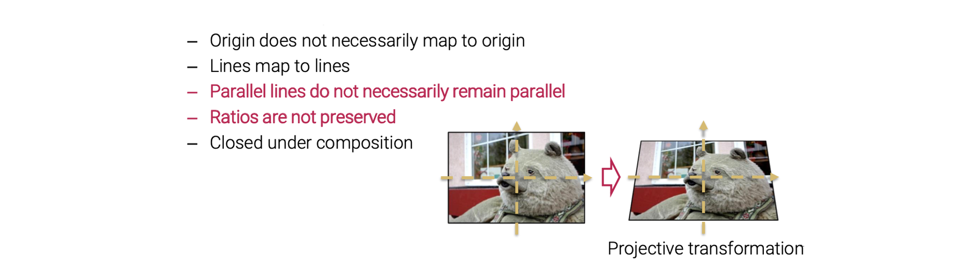여기서도 원점이 반드시 원점에 mapping 되지 않고, line은 line에 mapping 된다. 여기까지는 affine transformation과 같다. 여기서 가장 중요한건 parallel line은 반드시 parallel로 남지 않고, ratio도 보존되지 않는다. 위의 예시를 보면 세로선은 평행이 깨지고, 가로선의 길이는 달라진 것을 볼 수 있다. 이 또한 마찬가지로 composition에 close 되어있어서 projective transformation들의 조합이 여전히 projective transformation이다.

Projective transformation은 평면의 2D projection에 대한 warping을 설명하는 가장 일반적인 transformation이다. 이것이 가장 유용한 이유는 관계성을 쉽게 설명할 수 있기 때문이다.
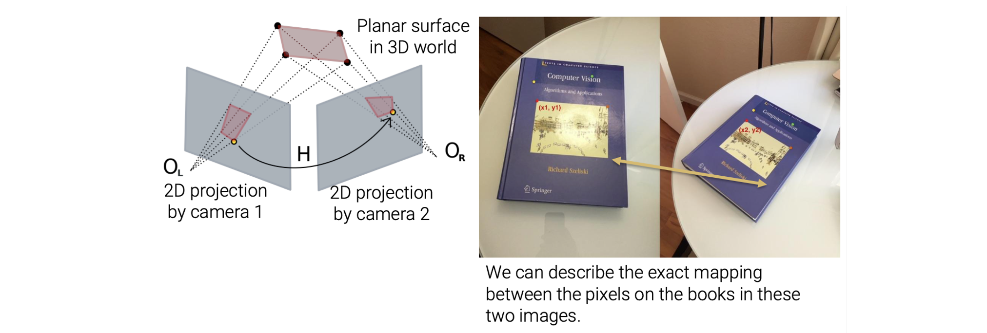예를 들어 3D 세계에 평면이 존재한다고 해보자. 우리는 2개의 카메라를 이용해서 다른 평면을 얻을 수 있다. 그러면 이제 얻어진 평면으로부터 projective transformation을 이용해서 pixel간 정확한 mapping을 설명할 수 있다.

2D Image Transformations

다음의 diagram은 서로 다른 2D transformation을 요약해서 보여주는 것이다.
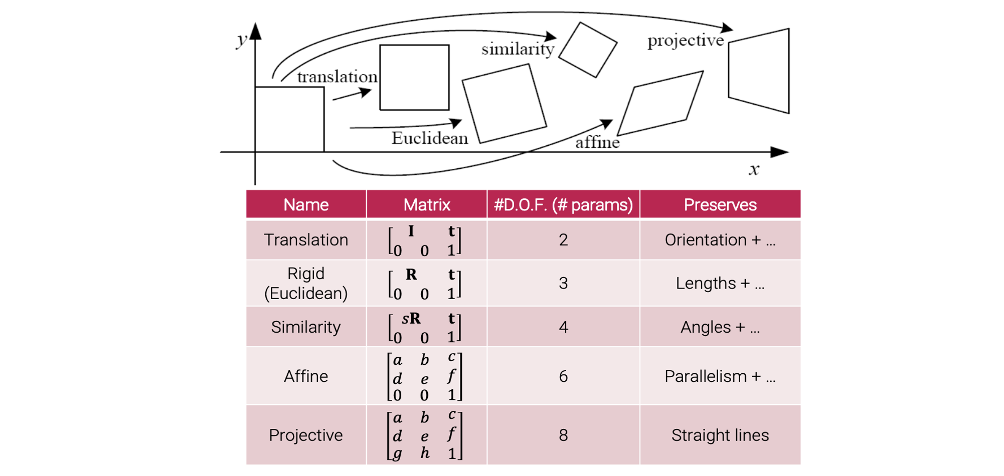Translation은 $3\times 3$ matrix로 나타내고 여기서 $I$ 는 $2\times 2$ identity matrix이고, $t$ 는 얼마나 이동시킬지에 대한 2차원 vector다. Translation은 x, y축으로 얼마나 이동할지에 대해서 2개의 parameter로 설명이 가능하다.

Rigid-body는 $3\times 3$ matrix로 나타내고 여기서 $R$ 은 $2\times 2$ rotation matrix이고, 3개의 parameter로 설명이 가능하다. 하나는 rotation angle, 나머지 2개는 translation에 대한 것이다.

Similarity는 $3\times 3$ matrix로 나타내고 $s$ 는 uniform scaling factor이다. 이 transformation은 $s$ 를 추가해서 4개의 parameter로 설명이 가능하다.

Affine은 $3\times 3$ matrix로 나타내고 6개의 parameter로 설명이 가능하다.

Projective는 $3\times 3$ matrix로 나타내고 8개의 parameter로 설명이 가능하다.

Projective transformation은 straight line들을 보존한다. Affine transformation은 parallelism과 straight line 모두에 대해서 보존이 가능하다. Similar transformation은 여기에 angle도 보존하고, rigid-body transformation은 여기에 length를 보존한다. 마지막으로 translation은 orientation까지 보존하게 된다.

JAEYOON SIM

평범한 공대생의 일상 (글을 잘 못 쓰는 사람이라 열심히 쓰려고 노력 중입니다^^)

이전 포스트

[계산사진학] Image Blending

다음 포스트

[계산사진학] Image Warping 2

1개의 댓글

홍순원

2022년 12월 22일

좋은 자료 감사합니당!

답글 달기