Introduce
이번 과제는 주어진 이미지 데이터셋을 Logistic Regression과 KNN을 이용해서 해결하는 과제와
스스로 이미지 데이터셋을 준비해서 분류 알고리즘을 만들어보는 과제로 이루어져 있다.
Obstacles
이미지 데이터를 모델에 학습시키기 위해서 준비를 하는 과정을 처음 하다보니 지금까지는 주어진 데이터를 받기만 했었다는 것을 실감할 수 있었다. 동시에 좋은 데이터를 준비한다는 것이 중요하다는 것을 느낄 수 있었다.
또한 분류의 정확도를 높이기 위한 최적화의 과정이 상당한 시간 소요가 걸린다는 것을 알게 되었다. 그간은 수업에서 어느정도는 주어진 보기?들에서 선택하는 것이었다면 이번에 Knn에서 활용할 거리 함수를 알아보고 준비하는 것은 모델에 대한 이해와 수학적인 지식이 요구되는 일이라는 것을 아는 기회가 되었다.
colab에서 진행을 하였기에 정말 편리했지만 만약 내가 직접 세팅을 해야하는 상황이 온다면 살짝 두렵다.
Image Classification
Dataset 준비하기
# 깃허브에서 데이터셋 다운로드하기
!git clone https://github.com/ndb796/Scene-Classification-Dataset
# 폴더 안으로 이동
%cd Scene-Classification-Dataset
import os
import pandas as pd
path = 'train-scene classification/'
# 전체 이미지 개수 출력하기
file_list = os.listdir(path + 'train/')
print('전체 이미지의 개수:', len(file_list))
# 학습 이미지 확인하기
dataset = pd.read_csv(path + 'train.csv')
print('학습 이미지의 개수:', len(dataset))
print('학습 이미지별 클래스 정보')
dataset.head()import numpy as np
import matplotlib.pyplot as plt
%matplotlib inline
from skimage.transform import resize
from PIL import Image
import numpy as np
img = Image.open(path + 'train/' + file_list[0])
img = np.asarray(img)
img = resize(img, (64, 64, 3))
print('이미지의 해상도:', img.shape)
# print(img)
# 이미지 출력하기
plt.imshow(img)
plt.show()from sklearn.model_selection import train_test_split
train_dataset, val_dataset = train_test_split(dataset, test_size=0.2)
print('학습 데이터셋 크기:', len(train_dataset))
print('검증 데이터셋 크기:', len(val_dataset))X_train = []
y_train = []
for index, row in train_dataset.iterrows():
#index, row['image_name'], row['label'])
img = Image.open(path + 'train/' + row['image_name'])
img = np.asarray(img)
img = resize(img, (64, 64, 3))
X_train.append(img)
y_train.append(row['label'])
X_train = np.array(X_train)
y_train = np.array(y_train)
X_val = []
y_val = []
for index, row in val_dataset.iterrows():
#index, row['image_name'], row['label'])
img = Image.open(path + 'train/' + row['image_name'])
img = np.asarray(img)
img = resize(img, (64, 64, 3))
X_val.append(img)
y_val.append(row['label'])
X_val = np.array(X_val)
y_val = np.array(y_val)
X_train = X_train.reshape(13627,12288)
X_val = X_val.reshape(3407,12288)
X_train.shape # (13627, 12288)LogisticRegression
from sklearn.linear_model import LogisticRegression
import time

start_time = time.time() # 시작 시간

model = LogisticRegression(multi_class="multinomial", solver="lbfgs", max_iter=10)
model.fit(X_train, y_train)

print("소요된 시간(초 단위):", time.time() - start_time) # 실행 시간
from sklearn.metrics import accuracy_score
y_pred = model.predict(X_train)
train_acc = accuracy_score(y_train, y_pred)
print('학습 데이터셋 정확도:', train_acc)
y_pred = model.predict(X_val)
val_acc = accuracy_score(y_val, y_pred)
print('검증 데이터셋 정확도:', val_acc)
print('클래스:', model.classes_)
print('반복 횟수:', model.n_iter_)
print('학습된 가중치 크기:', model.coef_.shape)Data Augmentation : Shift, Flip
from scipy.ndimage.interpolation import shift

def shift_image(image, dx, dy):
    image = image.reshape((64, 64, 3))
    # dy, dx는 각각 너비, 높이 기준으로 이동할 크기
    shifted_image = shift(image, [dy, dx, 0])
    return shifted_image.reshape([-1])

def horizontal_flip(image):
    image = image.reshape((64, 64, 3))
    # 수직 반전(vertical flip): axis=0, 수평 반전(horizontal flip): axis=1
    flipped_image = np.flip(image, axis=1)
    return flipped_image.reshape([-1])
X_train_augmented = [image for image in X_train]
y_train_augmented = [label for label in y_train]
# 이미지를 하나씩 확인하며 변형된 이미지 추가
cnt = 0
for image, label in zip(X_train, y_train):
dx = np.random.uniform(1, 3)
dy = np.random.uniform(1, 3)
X_train_augmented.append(shift_image(image, dx, dy))
y_train_augmented.append(label)
X_train_augmented = np.array(X_train_augmented)
y_train_augmented = np.array(y_train_augmented)
# 증진된 데이터들을 섞기(shuffle)
shuffle_idx = np.random.permutation(len(X_train_augmented))
X_train_augmented = X_train_augmented[shuffle_idx]
y_train_augmented = y_train_augmented[shuffle_idx]LR training and test
from sklearn.preprocessing import StandardScaler

scaler = StandardScaler()
scaler.fit(X_train)
#scaler.fit(X_train_augmented)

#X_train_augmented = scaler.transform(X_train_augmented)
X_val = scaler.transform(X_val)
X_train = scaler.transform(X_train)
model = LogisticRegression(multi_class="multinomial",solver="lbfgs", max_iter=20)
model.fit(X_train, y_train)
y_pred = model.predict(X_train)
train_acc = accuracy_score(y_train, y_pred)
print('학습 데이터셋 정확도:', train_acc)
y_pred = model.predict(X_val)
val_acc = accuracy_score(y_val, y_pred)
print('검증 데이터셋 정확도:', val_acc)
print('클래스:', model.classes_)
print('반복 횟수:', model.n_iter_)
print('학습된 가중치 크기:', model.coef_.shape)
학습 데이터셋 정확도: 0.5885374623908417
검증 데이터셋 정확도: 0.5518051071323745
클래스: [0 1 2 3 4 5]
반복 횟수: [20]
학습된 가중치 크기: (6, 12288)Knn Model
거리 함수로 L1L2의 평균을 사용하는 함수와 hassant거리를 사용하는 함수를 추가해주었다.
from collections import Counter


class kNearestNeighbors(object):
    def __init__(self):
        pass

    def train(self, X_train, y_train):
        self.X_train = X_train
        self.y_train = y_train

    def L1_distance(self, x):
        distances = np.sum(np.abs(self.X_train - x), axis=1)
        return distances

    def L2_distance(self, x):
        distances = np.sqrt(np.sum(np.square(self.X_train - x), axis=1))
        return distances

    def L1L2_distance(self, x):
        distances = np.sqrt(np.sum(np.square(self.X_train - x), axis=1)) + np.sum(np.abs(self.X_train - x), axis=1)
        distances = 1/2 * distances
        return distances

    def hassant_distance(self, v1, v2):
        total = 0
        for xi, yi in zip(v1, v2):
            min_val = min(xi, yi)
            max_val = max(xi, yi)
            if min_val >= 0:
                total += 1 - (1 + min_val)/(1 + max_val)
            else:
                total += 1 - (1 + min_val + abs(min_val))/(1 + max_val + abs(max_val))
        return total

    def predict(self, X_val, k, distance):
        num_val = X_val.shape[0]
        y_pred = np.zeros((num_val), dtype=int)

        for i in range(num_val):
            shortest = []
            # 각 검증 이미지(i번째 이미지)마다 모든 학습 이미지와의 거리 계산
            if distance == 'L1':
                distances = self.L1_distance(X_val[i, :])
            if distance == 'L2':
                distances = self.L2_distance(X_val[i, :])
            if distance == 'L1L2mean':
                distances = self.L1L2_distance(X_val[i, :])
            if distance == 'hassant':
                distances = []
                for h in range(13627):
                    distances.append(self.hassant_distance(X_train[h], X_val[i, :]))

            min_indices = np.argsort(distances) # 가까운 학습 이미지 순으로 정렬
            for j in range(k): # 가장 가까운 k개의 학습 이미지의 인덱스를 확인해 레이블 정보 기록
                shortest.append(self.y_train[min_indices[j]])
            y_pred[i] = Counter(shortest).most_common(1)[0][0] # 가장 많이 등장한 레이블(label) 계산
        return y_pred
Knn은 예측에 너무 많은 시간이 걸려서 val dataset의 크기를 조절해줄 필요가 있다.
start_time = time.time() # 시작 시간

knn = kNearestNeighbors()
knn.train(X_train, y_train)

number = 200
X_val_small = X_val[:number]
y_val_small = y_val[:number]

y_pred = knn.predict(X_val_small, k=14, distance='L1L2mean')
val_acc = accuracy_score(y_val_small, y_pred)
print('검증 데이터셋 정확도:', val_acc)

print("소요된 시간(초 단위):", time.time() - start_time) # 실행 시간
print("====================================================")

max_cnt = 5

# 이미지들이 들어갈 수 있는 그림(figure) 생성
fig, axes = plt.subplots(1, max_cnt)
fig.set_size_inches(12, 4)
fig.tight_layout()

for ax, image, label, pred in zip(axes, X_val_small[:max_cnt], y_val_small[:max_cnt], y_pred[:max_cnt]):
    ax.imshow(np.reshape(image, (64, 64, 3))) # 출력할 때는 이미지 해상도에 맞게 재변형
    ax.axis('off')
    ax.set_title(f'True label: {label}\nPredicted label: {pred}')

검증 데이터셋 정확도: 0.545
소요된 시간(초 단위): 324.29480934143066
Custom dataset 사용하기
Data 준비하기
!wget --no-check-certificate \
https://storage.googleapis.com/mledu-datasets/cats_and_dogs_filtered.zip \
-O /tmp/cats_and_dogs_filtered.zip
import os
import zipfile
local_zip = '/tmp/cats_and_dogs_filtered.zip'
zip_ref = zipfile.ZipFile(local_zip, 'r')
zip_ref.extractall('/tmp')
zip_ref.close()
base_dir = '/tmp/cats_and_dogs_filtered'
train_dir = os.path.join(base_dir, 'train')
validation_dir = os.path.join(base_dir, 'validation')
train_cats_dir = os.path.join(train_dir, 'cats')
train_dogs_dir = os.path.join(train_dir, 'dogs')
print(train_cats_dir) # /tmp/cats_and_dogs_filtered/train/cats
print(train_dogs_dir) # /tmp/cats_and_dogs_filtered/train/dogs
validation_cats_dir = os.path.join(validation_dir, 'cats')
validation_dogs_dir = os.path.join(validation_dir, 'dogs')
print(validation_cats_dir) # /tmp/cats_and_dogs_filtered/validation/cats
print(validation_dogs_dir) # /tmp/cats_and_dogs_filtered/validation/dogs그려보자.
train_cat_fnames = os.listdir(train_cats_dir)
train_dog_fnames = os.listdir(train_dogs_dir)

print(train_cat_fnames[:5]) # ['cat.464.jpg', 'cat.870.jpg', 'cat.283.jpg', 'cat.883.jpg', 'cat.463.jpg']
print(train_dog_fnames[:5]) # ['dog.451.jpg', 'dog.115.jpg', 'dog.466.jpg', 'dog.902.jpg', 'dog.839.jpg']
import matplotlib.image as mpimg
import matplotlib.pyplot as plt
%matplotlib inline
nrows, ncols = 4, 4
pic_index = 0
fig = plt.gcf()
fig.set_size_inches(ncols*3, nrows*3)
pic_index+=8
next_cat_pix = [os.path.join(train_cats_dir, fname)
for fname in train_cat_fnames[ pic_index-8:pic_index]]
next_dog_pix = [os.path.join(train_dogs_dir, fname)
for fname in train_dog_fnames[ pic_index-8:pic_index]]
for i, img_path in enumerate(next_cat_pix+next_dog_pix):
sp = plt.subplot(nrows, ncols, i + 1)
sp.axis('Off')
img = mpimg.imread(img_path)
plt.imshow(img)
plt.show()
print(next_cat_pix) # ['/tmp/cats_and_dogs_filtered/train/cats/cat.464.jpg', '/tmp/cats_and_dogs_filtered/train/cats/cat.870.jpg',이미지 데이터를 가져와서 전처리를 하고 정리해보자.
from tensorflow.keras.preprocessing.image import ImageDataGenerator

train_datagen = ImageDataGenerator( rescale = 1.0/255. )
test_datagen  = ImageDataGenerator( rescale = 1.0/255. )

train_generator = train_datagen.flow_from_directory(train_dir,
                                                  batch_size=20,
                                                  class_mode='binary',
                                                  target_size=(150, 150))
validation_generator =  test_datagen.flow_from_directory(validation_dir,
                                                       batch_size=20,
                                                       class_mode  = 'binary',
                                                       target_size = (150, 150))
CNN Model training and validate
import tensorflow as tf

model = tf.keras.models.Sequential([
  tf.keras.layers.Conv2D(16, (3,3), activation='relu', input_shape=(150, 150, 3)),
  tf.keras.layers.MaxPooling2D(2,2),
  tf.keras.layers.Conv2D(32, (3,3), activation='relu'),
  tf.keras.layers.MaxPooling2D(2,2),
  tf.keras.layers.Conv2D(64, (3,3), activation='relu'),
  tf.keras.layers.MaxPooling2D(2,2),
  tf.keras.layers.Flatten(),
  tf.keras.layers.Dense(512, activation='relu'),
  tf.keras.layers.Dense(1, activation='sigmoid')
])

model.summary()
from tensorflow.keras.optimizers import RMSprop
model.compile(optimizer=RMSprop(lr=0.001),
loss='binary_crossentropy',
metrics = ['accuracy'])
history = model.fit(train_generator,
validation_data=validation_generator,
steps_per_epoch=100,
epochs=15,
validation_steps=50,
verbose=2)import matplotlib.pyplot as plt
acc = history.history['accuracy']
val_acc = history.history['val_accuracy']
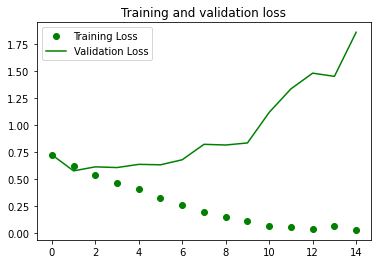
loss = history.history['loss']
val_loss = history.history['val_loss']
epochs = range(len(acc))
plt.plot(epochs, acc, 'bo', label='Training accuracy')
plt.plot(epochs, val_acc, 'b', label='Validation accuracy')
plt.title('Training and validation accuracy')
plt.legend()
plt.figure()
plt.plot(epochs, loss, 'go', label='Training Loss')
plt.plot(epochs, val_loss, 'g', label='Validation Loss')
plt.title('Training and validation loss')
plt.legend()
plt.show()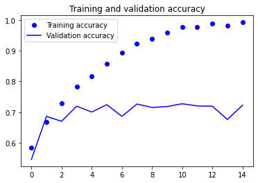

chords & code // harmony with structure