[Dev Course Weekly실습]#5, multilayer perceptron with mnist

Introduce

9주차 5번째날의 실습과제는 mnist 데이터를 심층 신경망을 이용해서 처리해보는 것이다.
프레임워크로는 tensorflow와 pytorch를 둘다 사용해야 한다. 조건은 다음과 같다.

[1/2번: CPU 사용]
1.첨부된 multilayer perceptron을 수행하고, 이해해봅시다.
2.2가지 이상 제공된 multilayer perceptron 성능 향상 방법을 제안하고, 결과를 확인 해봅시다.

[3/4번: GPU 사용, Colab 사용 권장(아나콘다를 사용한 로컬 GPU 환경을 사용해도 무방)]
3.2번의 모델을 GPU 연산으로 학습하세요.
4.3번의 PyTorch로 구현된 모델을 TensorFlow로 동일하게 구현해보세요.

Obstacles

가장 애를 먹었던 부분은 학습을 수행할때마다 colab을 초기화 시켜주어야 한다는 것이었다.
epoch값을 바꾸어 학습을 반복할수록 w값은 계속해서 업데이트가 되기 때문에
epoch값에 대한 정확한 학습률을 측정하기 위해선 런타임을 초기화 해줄 필요가 있었다.
물론 이 부분은 내가 pytorch에 익숙하지 않아서 생긴 문제이기도 하다.
tensorflow에서는 epoch를 크게해서 모델을 학습하고 과적합이 발생하기 시작한 시점에
최적의 모델을 저장하여 학습을 조기종료 하는 방법을 사용했다.
pytorch모델은 이미 만들어진 폼에서 파라미터만을 조정하는 과업이었기에 적극적으로 코드를 고치지는 않았다.

만약 pytorch에서 early stop을 사용하고 싶다면 아래 글을 참조하면 좋을듯하다.
https://quokkas.tistory.com/37

pytorch base

Load and Visualize the Data

import torch
import numpy as np
from torchvision import datasets
import torchvision.transforms as transforms

# number of subprocesses to use for data loading
num_workers = 0
# how many samples per batch to load
batch_size = 20

# convert data to torch.FloatTensor
transform = transforms.ToTensor()

# choose the training and test datasets
train_data = datasets.MNIST(root='data', train=True,
                                   download=True, transform=transform)
test_data = datasets.MNIST(root='data', train=False,
                                  download=True, transform=transform)

# prepare data loaders
train_loader = torch.utils.data.DataLoader(train_data, batch_size=batch_size,
    num_workers=num_workers)
test_loader = torch.utils.data.DataLoader(test_data, batch_size=batch_size, 
    num_workers=num_workers)

Visualize a Batch of Training Data

import matplotlib.pyplot as plt
%matplotlib inline
    
# obtain one batch of training images
dataiter = iter(train_loader)
images, labels = dataiter.next()
images = images.numpy()

# plot the images in the batch, along with the corresponding labels
fig = plt.figure(figsize=(25, 4))
for idx in np.arange(20):
    ax = fig.add_subplot(2, 20/2, idx+1, xticks=[], yticks=[])
    ax.imshow(np.squeeze(images[idx]), cmap='gray')
    # print out the correct label for each image
    # .item() gets the value contained in a Tensor
    ax.set_title(str(labels[idx].item()))

Define the Network Architecture

import torch.nn as nn
import torch.nn.functional as F

class Net(nn.Module):
    def __init__(self):
        super(Net, self).__init__()
        self.fc1 = nn.Linear(28*28, 128)
        self.fc2 = nn.Linear(128, 128)
        self.fc3 = nn.Linear(128,10)
        self.dropout = nn.Dropout(0.5)

    def forward(self, x):
        # image input을 펼쳐준다.
        x = x.view(-1, 28*28)

        # 은닉층을 추가하고 활성화 함수로 relu 사용
        x = F.relu(self.fc1(x))
        x = self.dropout(x)

        # 은닉층을 추가하고 활성화 함수로 relu 사용
        x = F.relu(self.fc2(x))
        x = self.dropout(x)

        # 출력층 추가
        x = self.fc3(x)
        return x

# initialize the NN / 모델 확인
model = Net()
model = model.to('cuda')
print(model)

Specify Loss Function and Optimizer

## Specify loss and optimization functions

# specify loss function
criterion = nn.CrossEntropyLoss()

# specify optimizer
optimizer = torch.optim.Adam(model.parameters())

Train the Network

# number of epochs to train the model
n_epochs = 20  # suggest training between 10-50 epochs

model.train() # prep model for training

for epoch in range(n_epochs):
    # monitor training loss
    train_loss = 0.0
    
    ###################
    # train the model #
    ###################
    for data, target in train_loader:
        # clear the gradients of all optimized variables
        optimizer.zero_grad()
        data, target = data.to('cuda') , target.to('cuda')
        # forward pass: compute predicted outputs by passing inputs to the model
        output = model(data)
        # calculate the loss
        loss = criterion(output, target)
        # backward pass: compute gradient of the loss with respect to model parameters
        loss.backward()
        # perform a single optimization step (parameter update)
        optimizer.step()
        # update running training loss
        train_loss += loss.item()*data.size(0)
        
    # print training statistics 
    # calculate average loss over an epoch
    train_loss = train_loss/len(train_loader.dataset)

    print('Epoch: {} \tTraining Loss: {:.6f}'.format(
        epoch+1, 
        train_loss
        ))

Epoch: 1 	Training Loss: 0.459142
Epoch: 2 	Training Loss: 0.276919
Epoch: 3 	Training Loss: 0.239554
Epoch: 4 	Training Loss: 0.219908
Epoch: 5 	Training Loss: 0.209204
Epoch: 6 	Training Loss: 0.198766
Epoch: 7 	Training Loss: 0.190210
Epoch: 8 	Training Loss: 0.184474
Epoch: 9 	Training Loss: 0.179768
Epoch: 10 	Training Loss: 0.169017
Epoch: 11 	Training Loss: 0.169036
Epoch: 12 	Training Loss: 0.162453
Epoch: 13 	Training Loss: 0.164836
Epoch: 14 	Training Loss: 0.156412
Epoch: 15 	Training Loss: 0.156915
Epoch: 16 	Training Loss: 0.158710
Epoch: 17 	Training Loss: 0.152928
Epoch: 18 	Training Loss: 0.152353
Epoch: 19 	Training Loss: 0.149320
Epoch: 20 	Training Loss: 0.146735

Test The Trained Network

# initialize lists to monitor test loss and accuracy
test_loss = 0.0
class_correct = list(0. for i in range(10))
class_total = list(0. for i in range(10))

model.eval() # prep model for *evaluation*

for data, target in test_loader:
    if len(target.data) != batch_size:
          break
    data, target = data.to('cuda') , target.to('cuda')
    # forward pass: compute predicted outputs by passing inputs to the model
    output = model(data)
    # calculate the loss
    loss = criterion(output, target)
    # update test loss 
    test_loss += loss.item()*data.size(0)
    # convert output probabilities to predicted class
    _, pred = torch.max(output, 1)
    # compare predictions to true label
    correct = np.squeeze(pred.eq(target.data.view_as(pred)))
    # calculate test accuracy for each object class
    for i in range(batch_size):
        label = target.data[i]
        class_correct[label] += correct[i].item()
        class_total[label] += 1

# calculate and print avg test loss
test_loss = test_loss/len(test_loader.dataset)
print('Test Loss: {:.6f}\n'.format(test_loss))

for i in range(10):
    if class_total[i] > 0:
        print('Test Accuracy of %5s: %2d%% (%2d/%2d)' % (
            str(i), 100 * class_correct[i] / class_total[i],
            np.sum(class_correct[i]), np.sum(class_total[i])))
    else:
        print('Test Accuracy of %5s: N/A (no training examples)' % (classes[i]))

print('\nTest Accuracy (Overall): %2d%% (%2d/%2d)' % (
    100. * np.sum(class_correct) / np.sum(class_total),
    np.sum(class_correct), np.sum(class_total)))

Test Loss: 0.100577

Test Accuracy of     0: 98% (970/980)
Test Accuracy of     1: 99% (1128/1135)
Test Accuracy of     2: 97% (1006/1032)
Test Accuracy of     3: 96% (979/1010)
Test Accuracy of     4: 97% (962/982)
Test Accuracy of     5: 96% (864/892)
Test Accuracy of     6: 96% (925/958)
Test Accuracy of     7: 97% (1005/1028)
Test Accuracy of     8: 96% (936/974)
Test Accuracy of     9: 95% (962/1009)

Test Accuracy (Overall): 97% (9737/10000)

Tensorflow base

Prepare the Data

데이터를 train_loader에서 받아와 numpy로 바꿔주기로 했다.

from tensorflow import keras
import tensorflow as tf
import torch
import numpy as np

from torchvision import datasets
import torchvision.transforms as transforms

# number of subprocesses to use for data loading
num_workers = 0
# how many samples per batch to load
#batch_size = 20

# convert data to torch.FloatTensor
transform = transforms.ToTensor()

# choose the training and test datasets
train_data = datasets.MNIST(root='data', train=True,
                                   download=True, transform=transform)
test_data = datasets.MNIST(root='data', train=False,
                                  download=True, transform=transform)

for data, target in train_loader:
  train_input = data
  train_target = target

for data, target in test_loader:
  test_input = data
  test_target = target
  
train_input = train_input.numpy()
train_target = train_target.numpy()
test_input = test_input.numpy()
test_target = test_target.numpy()

train_input.shape # (60000, 1, 28, 28)
train_target.shape # (60000,)

train_input = train_input.squeeze(axis=1)
test_input = test_input.squeeze(axis=1)

Preprocessing

train_scaled = train_input / 255.0
test_scaled = test_input / 255.0

from sklearn.model_selection import train_test_split
train_scaled, val_scaled, train_target, val_target = train_test_split(train_scaled, train_target, test_size=0.2, random_state=42)

Making Model

model = keras.Sequential()
model.add(keras.layers.Flatten(input_shape=(28,28)))
model.add(keras.layers.Dense(128, activation='relu'))
model.add(keras.layers.Dropout(0.5))
model.add(keras.layers.Dense(128, activation='relu'))
model.add(keras.layers.Dropout(0.5))
model.add(keras.layers.Dense(10, activation='softmax'))

model.summary()

Training

model.compile(optimizer='adam', loss='sparse_categorical_crossentropy', metrics='accuracy')

checkpoint_cb = keras.callbacks.ModelCheckpoint('best-model.h5')
early_stopping_cb = keras.callbacks.EarlyStopping(patience=7, restore_best_weights=True)

history = model.fit(train_scaled, train_target, epochs=50, verbose=0, validation_data=(val_scaled, val_target), callbacks=[checkpoint_cb, early_stopping_cb])
model = keras.models.load_model('best-model.h5')

print(early_stopping_cb.stopped_epoch)

import matplotlib.pyplot as plt
import seaborn as sns

plt.plot(history.history['loss'])
plt.plot(history.history['val_loss'])
plt.xlabel('epoch')
plt.ylabel('loss')
plt.legend(['train', 'val'])
plt.show()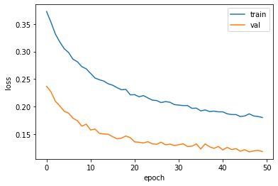

Test

test_labels = np.argmax(model.predict(test_scaled), axis=-1)
print(np.mean(test_labels == test_target))