Key words
AutoEncoder, Latent(잠재) 벡터, DAE(Denoising AutoEncoder), 이상치 탐지(Anomaly Detection)
오늘은 배운 개념이 매우 심플하다.
1. AutoEncoder란?
AutoEncoder (오토인코더)는 입력 데이터를 저차원의 벡터로 압축한 뒤 원래 크기의 데이터로 복원하는 신경망이다. 이미지를 보자.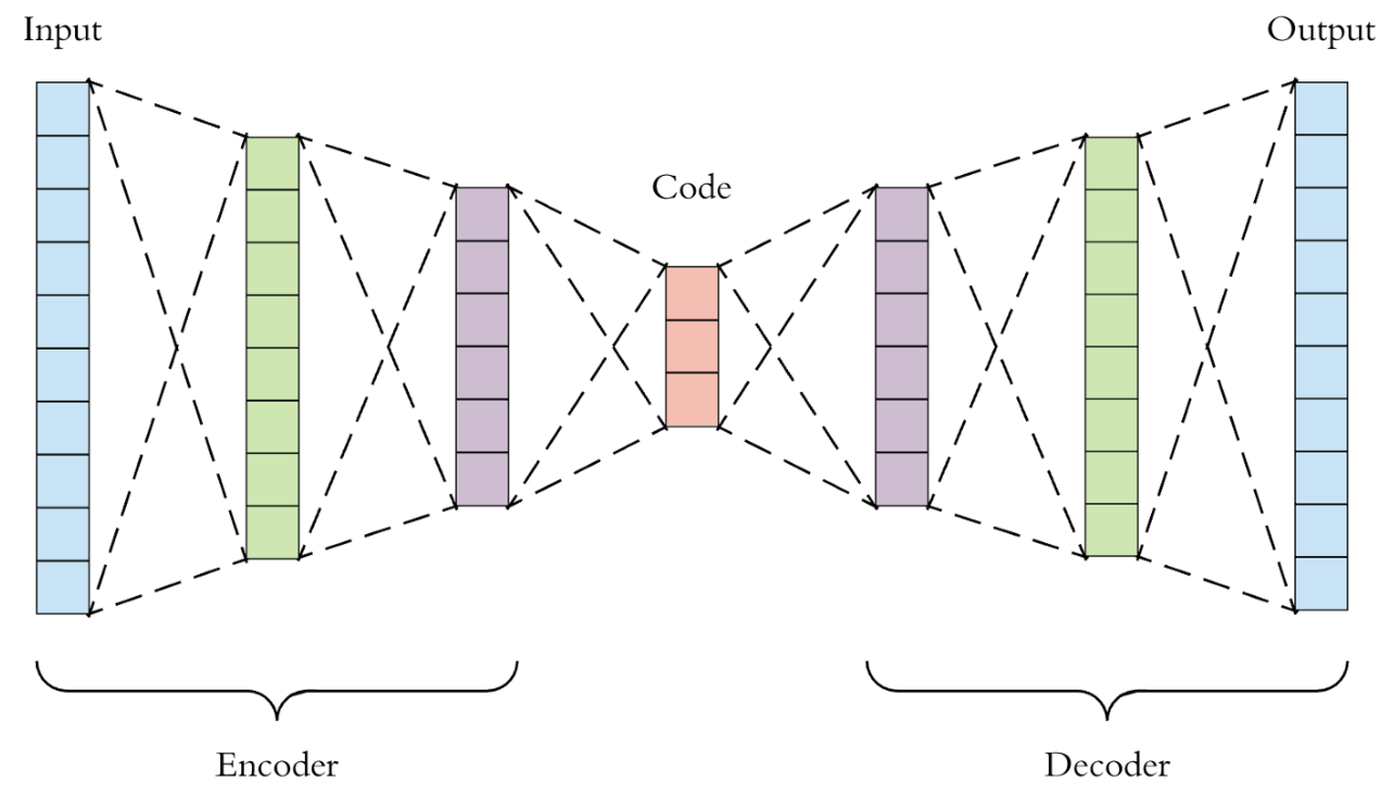
- 어제 보았던
U-net구조랑 비슷하게 보인다.
- 어제 보았던
- 여기서 가장 중요한 건 저 가운데의
code부분이다. 저 벡터를 Latent vector (잠재 벡터)라고 하는데, 원본 데이터보다 차원이 작으면서도 원본 데이터의 특징을 잘 보존하고 있는 벡터라는 의미가 있다.- AutoEncoder는 사실상 이 잠재 벡터를 잘 얻기 위한 방법이라고 생각해도 될 정도라고 한다.
- 관련하여 Manifold Learning 자료 참고.
- 이 오토 인코더가 의미가 있는 건 인코딩한 데이터를 다시 디코딩하는 과정에서 원본 데이터의 특징을 최대한 보존하는 Latent 벡터를 학습할 수 있게 된다는 것 기억!!!!
AutoEncoder의 대표적인 활용은 다음 세 가지가 있다.
- 차원 축소(Dimensionality Reduction)와 데이터 압축
- 데이터 노이즈 제거(Denoising)
- 이상치 탐지(Anomaly Detection)
중요!!
- U-net 등이 지도학습이었다면 이 오토 인코더는 비지도학습이다! 학습 시 정답 데이터(=레이블)를 안 넣어준다!
- 산불이 났는지를 예측하려고 할 때 일반적인 산의 모습을 학습 시킨 후 산불이 난 모습이 이상치다! 라고 해서 감지하는 모델을 만들 수 있는데, 이때 지도학습이면 산불이 난 산 이미지를 대량으로 넣어줘야 한다. 근데 현실적으로 산불 이미지를 대량으로 확보하기는 어려울 수 있다. 그럴 때 이런 오토인코더를 써주기도 한다고 한다. 오토인코더는 정상 이미지만 넣어주면 되기 때문에 그것만 가지고 이상치 탐지를 할 수 있기 때문이다.
- 이것 역시 latent vector 덕분이라고 할 수 있을 것 같다.
2. AutoEncoder의 활용
[기본 활용]
LATENT_DIM = 64

class Autoencoder(Model):
    def __init__(self, latent_dim):
        super(Autoencoder, self).__init__()
        self.latent_dim = latent_dim
        self.encoder = tf.keras.Sequential([
            layers.Flatten(),
            layers.Dense(latent_dim, activation='relu'),
        ])
        self.decoder = tf.keras.Sequential([
            layers.Dense(784, activation='sigmoid'),
            layers.Reshape((28, 28))
        ])

    def call(self, x):
        encoded = self.encoder(x)
        decoded = self.decoder(encoded)
        return decoded

model = Autoencoder(LATENT_DIM)

model.compile(optimizer='adam', loss='mse')

model.fit(x_train, x_train,
          epochs=10,
          shuffle=True,
          validation_data=(x_test, x_test))
- 위 코드를 보면 알 수 있겠지만 인코더 부분과 디코더 부분이 있다.
- fit할 때 동일한 x_train 데이터만 넣는다는 점 기억!
[데이터 노이즈 제거]
- 노트에 있는 코드 그대로 옮겨오고 싶지만.. 그럴 수 없으니.. 필요하면 나중에 노트를 다시 보자.
- 순서만 좀 적어두면, 먼저 정상 이미지 데이터에 임의로 노이즈를 준다. 그리고 모델을 구축할 때 위 기본 활용과 같이 완전 연결신경망(Dense)을 사용하는게 아니라 합성곱 층을 이용한다. (검색 키워드: Convolutional AutoEncoder)
- Convolutional AutoEncoder을 이용하기 위해선
x_train = x_train[..., tf.newaxis]과 같이 훈련/검증 데이터에 임의의 채널을 하나더 추가해서 노이즈를 주어야 한다.
- Convolutional AutoEncoder을 이용하기 위해선
- fit할 때는 노이즈를 추가한 데이터와 정상 데이터를 넣어준다.
3. [이상치 탐지 (Anomaly Detection)]
- 이상치 탐지에 대해선 위에서 산불 탐지 모델 예시를 들었다.
- 오토 인코더를 활용해 이상치 탐지를 하는 원리는 아래와 같다.
AutoEncoder는 특정 데이터의 중요 특징, 즉 잠재 벡터를 바탕으로 다시 원본 데이터로 복원할 때에 발생하는 오류, 즉 복원 오류(Reconstruction Error)를 최소화 하도록 훈련됩니다.
정상 데이터로만 훈련한 뒤에 비정상 데이터셋을 복원한다면 복원 오류가 커질 것입니다. 복원 오류가 특정한 임계값을 초과하는 경우 해당 데이터를 비정상으로 판단할 수 있습니다. - 위의 산불 예시를 다시 가져와 보면, 일단 전제는 오토 인코더가 원본 데이터를 최대한 잘 보존할 수 있도록 인코딩을 한다. (그러니 복원 간에도 오류가 적어지는 것) 그런 후 정상적인 산의 모습을 담은 사진만을 가지고 학습을 한 모델이라면, 만약 산불이 난 산의 모습이 담긴 데이터가 들어와 이걸 기존에 학습한 모델로 복원하려고 할 때 오류가 올라가는 것이다.
- 다시 한번 강조!! 학습 시에는 정상 데이터만 학습해야 한다!!
이것도 코드 참고 필요시 노트나 구글링 해볼 것. 여기 옮겨두진 않겠다.
3. 실습한 것
오늘은 개념학습보다 실습 코드 적고 이해하는 데에 더 많은 시간과 어려움이 있었던 것 같다.
구글의 Quick Draw 데이터셋 중 고양이'를 스케치한 데이터를 활용한다.
- (손 낙서 데이터는 벡터 포맷으로 저장되어 있어서 비트맵 형태로 변환하여 사용해야 한다.)
이번 과제에서는 '고양이 스러움'을 학습하는 오토인코더 모델을 만들게 됩니다.
오토인코더의 Latent Vector가 고양이라는 스케치의 표현(Representation)을 담아낼 수 있도록 학습해보도록 합시다.
내가 공부하며 달아놓은 주석은 #=>와 같이 적거나 아예 여러 줄 주석처리를 해서 기록해두었다.
[데이터 불러오기]
import matplotlib.pyplot as plt
import json, glob
import numpy as np

---
from tensorflow.keras.utils import get_file

BASE_PATH = 'https://storage.googleapis.com/quickdraw_dataset/full/binary/'
path = get_file('cat', BASE_PATH + 'cat.bin')

---

import PIL # => 파이썬에서 이미지 분석/처리를 쉽게 할 수 있도록 도와주는 라이브러리임. (PIL = Python Imaging Library) - pilow module
from PIL import ImageDraw
from struct import unpack
from sklearn.model_selection import train_test_split
import tensorflow as tf

def load_drows(path, train_size=0.85):
    """
    데이터를 불러오는 역할을 하는 함수입니다.
    """

    x = []

    # 파일을 불러와 스케치를 하나하나 모읍니다.
    # 스케치가 15바이트 헤더로 시작하기 때문이 이런 부분을 전처리하여 줍니다.
    with open(path, 'rb') as f:
        while True:
            img = PIL.Image.new('L', (32, 32), 'white') # => PIL.Image.new(mode, size, color=0) // Creates a new image with the given mode and size. // L (8-bit pixels, black and white) 이외는 공식문서 참고하면 됨. https://pillow.readthedocs.io/en/stable/reference/Image.html
            draw = ImageDraw.Draw(img) # => 공식문서 https://pillow.readthedocs.io/en/stable/reference/ImageDraw.html?highlight=from%20PIL%20import%20ImageDraw
            header = f.read(15)
            if len(header) != 15:
                break

            # 낙서는 x,y 좌표로 구성된 획(stroke) 목록으로 되어 있고, 각 좌표는 분리되어 저장되어 있습니다.
            # 방금 위에서 생성한 ImageDraw 객체의 좌표 목록을 이용하기 위해 zip() 함수를 사용하여 합쳐주도록 합니다.
            strokes, = unpack('H', f.read(2)) # => 참고 https://docs.python.org/ko/3/library/struct.html

            for i in range(strokes):
                n_points, = unpack('H', f.read(2))
                fmt = str(n_points) + 'B'
                read_scaled = lambda: (p // 8 for
                                       p in unpack(fmt, f.read(n_points)))
                points = [*zip(read_scaled(), read_scaled())]
                draw.line(points, fill=0, width=2)
            img = tf.keras.preprocessing.image.img_to_array(img) # => img_to_array(img)에서 tf.keras.preprocessing.image.img_to_array(img)로 코드 변경함. 공식문서: https://www.tensorflow.org/api_docs/python/tf/keras/utils/img_to_array
            x.append(img)
    x = np.asarray(x) / 255
    return train_test_split(x, train_size=train_size)

# 입력받은 10만개의 고양이 낙서 데이터를 활용할 수 있다.
x_train, x_test = load_drows(path)

print(x_train.shape, x_test.shape) #=> (104721, 32, 32, 1) (18481, 32, 32, 1)
[오토 인코더 구축]
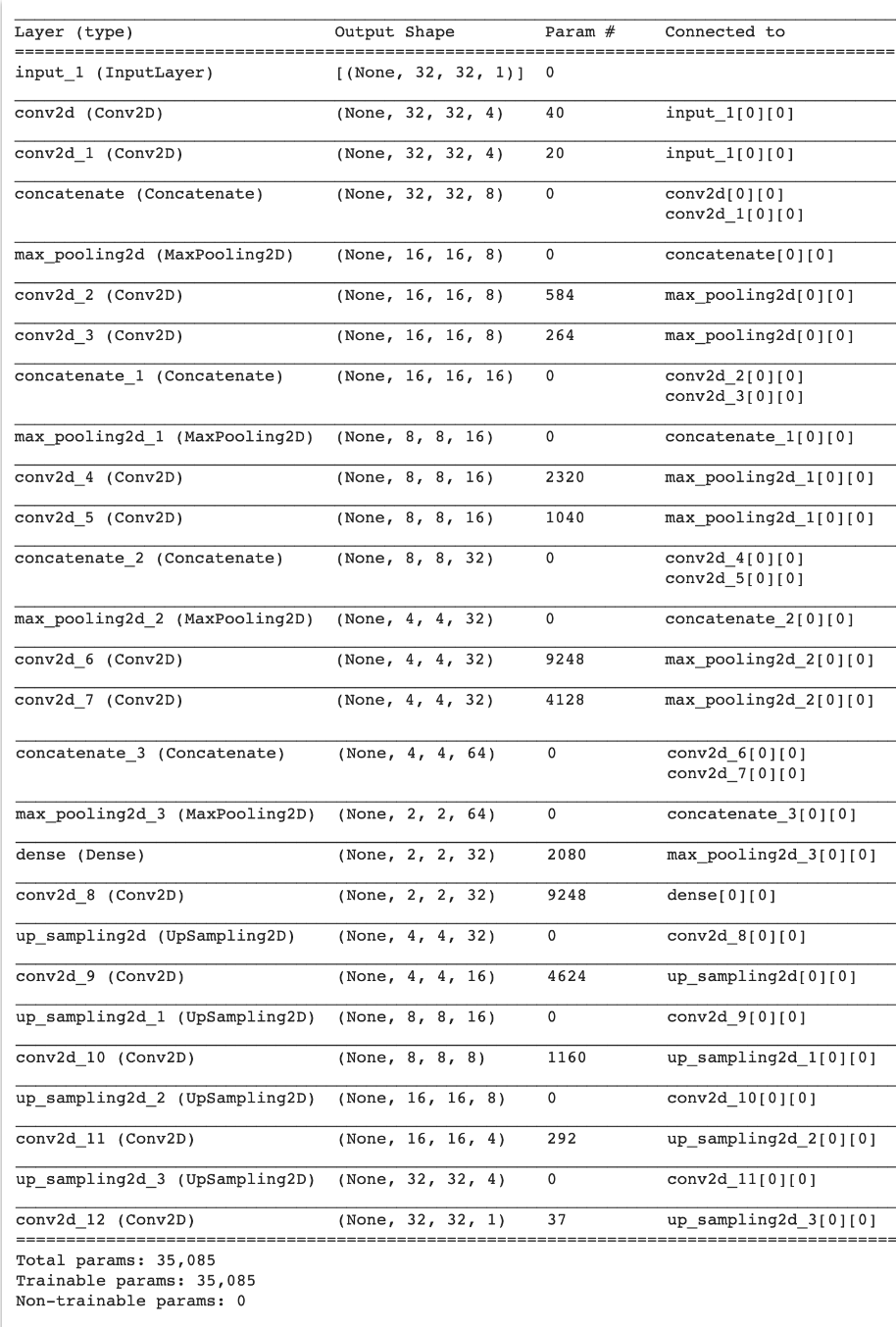
- 문제에서 주어졌던 모델 summary. 똑같이 인코더와 디코더를 구성해야 했다.
from re import X
from keras.layers import Input, Dense, Conv2D, MaxPooling2D, UpSampling2D, Reshape, Concatenate, Flatten, Lambda
from keras.models import Model
from keras.preprocessing.image import load_img, img_to_array, ImageDataGenerator
from keras.losses import binary_crossentropy, kullback_leibler_divergence
from keras import backend as K

def create_AE():
    input_img = Input(shape=(32, 32, 1))

    channels = 2
    x = input_img
    for i in range(4):
        channels *= 2 # => channels = channels * 2 = 4 // 변수 참고 https://corytips.tistory.com/162
        # 여기에 다운샘플링 할 수 있는 코드를 제작하세요.
        # 구조는 아래 첨부된 이미지를 참조하세요.
        # 사용할 함수 : Conv2D(activation='relu', padding='same'), Concatenate(), MaxPooling2D(padding='same')

        x_1 = Conv2D(channels, (3,3), activation='relu', padding='same')(x) # => 채널은 필터수 인거 잊지 말자 //  "same" 은 아웃풋이 원래 인풋과 동일한 길이를 갖도록 인풋을 패딩한다. (https://keras.io/ko/layers/convolutional/)
        x_2 = Conv2D(channels, (2,2), activation='relu', padding='same')(x)
        concatenate = Concatenate()([x_1, x_2]) # => Concatenate is used in a Sequential model, whereas concatenate is used in a Functional API이라곤 하는데, 이런 형태로 함수 뒤에 붙이니 되긴 하네. 출처: https://stackoverflow.com/questions/44720822/valueerror-with-concatenate-layer-keras-functional-api
        x = MaxPooling2D(2, padding='same')(concatenate)

    x = Dense(channels)(x)

    for i in range(4):
        # 여기에 업샘플링할 수 있는 코드를 제작 하세요.
        # 사용할 함수 : Conv2D(activation='relu', padding='same'), UpSampling2D()

        x = Conv2D(channels, (3, 3), activation='relu', padding='same')(x)
        x = UpSampling2D((2, 2))(x)

        channels //= 2 # => Channel을 2로 나눈 몫이 channel이 됨.

    decoded = Conv2D(1, (3, 3), activation='sigmoid', padding='same')(x)

    autoencoder = Model(input_img, decoded)
    autoencoder.compile(optimizer='adadelta', loss='binary_crossentropy')
    return autoencoder

autoencoder = create_AE()
autoencoder.summary()


'''
[기록 - 인코더 부분]
난 처음에 인코더 부분을 아래와 같이 직접 짜보고 이걸 for 문으로 어떻게 줄일 수 있을지 고민해보았다.
(for문의 i가 어떤 역할을 하는지, 어떻게 코드에 반영해야할지 고민을 많이 해봤는데, 도저히 들어갈 곳이 없어 찾아보니 그냥 똑같은 과정을 4번 반복한다는 의미로 쓸 수 있음을 배웠다.)

        conv2d = Conv2D(4, (3,3), activation='relu', padding='same')(x) # => "same" 은 아웃풋이 원래 인풋과 동일한 길이를 갖도록 인풋을 패딩한다. (https://keras.io/ko/layers/convolutional/)
        conv2d_1 = Conv2D(4, (3,3), activation='relu', padding='same')(conv2d)
        concatenate = Concatenate()([conv2d, conv2d_1]) # => Concatenate is used in a Sequential model, whereas concatenate is used in a Functional API이라곤 하는데, 이런 형태로 함수 뒤에 붙이니 되긴 하네. 출처: https://stackoverflow.com/questions/44720822/valueerror-with-concatenate-layer-keras-functional-api
        maxpool = MaxPooling2D((2,2), padding='same')(concatenate)

        conv2d_2 = Conv2D(8, (3,3), activation='relu', padding='same')(maxpool)
        conv2d_3 = Conv2D(8, (3,3), activation='relu', padding='same')(conv2d_2)
        concatenate_2 = Concatenate()([conv2d_2, conv2d_3])
        maxpool_2 = MaxPooling2D((2,2), padding='same')(concatenate_2)

        conv2d_4 = Conv2D(16, (3,3), activation='relu', padding='same')(maxpool_2)
        conv2d_5 = Conv2D(16, (3,3), activation='relu', padding='same')(conv2d_4)
        concatenate_3 = Concatenate()([conv2d_4, conv2d_5])
        maxpool_3 = MaxPooling2D((2,2), padding='same')(concatenate_3)

        conv2d_6 = Conv2D(32, (3,3), activation='relu', padding='same')(maxpool_3)
        conv2d_7 = Conv2D(32, (3,3), activation='relu', padding='same')(conv2d_6)
        concatenate_4 = Concatenate()([conv2d_6, conv2d_7])
        maxpool_4 = MaxPooling2D((2,2), padding='same')(concatenate_4)

-근데 이전 구조에 누적하는 위와 같은 방식이 아니라는 건, 문제에서 이미지로 주어진 모델 summary의 맨처음 conv2d 층이 'connected to'를 보면 둘다 'input_1[0][0]'인 것을 보고 동일한 인풋 데이터에서 합성곱을 해 concat한다는 걸 알았다.
-x_1과 x_2의 필터 사이즈가 다른 건 'Param #'으로 계산했다. 간단하게는 3*3*4 = 36 + 4 = 40 (편향 4개 포함) 이런 식으로 해도 되고, 아니면 이 수식을 참고해도 된다. (param_number = output_channel_number * (input_channel_number * kernel_height * kernel_width + 1))을 계산해보면 된다. 출처 - https://towardsdatascience.com/how-to-calculate-the-number-of-parameters-in-keras-models-710683dae0ca
-그리고 channel(필터 수)도 for loop에 의해 4, 8, 16, 32로 늘어나게 된다!!


[기록 - 디코더]
- 마찬가지로 디코더의 channel(필터 수)도 for loop에 의해 줄어듬. 위에서 채널 최종이 32였으니까 32, 16, 8, 4로 줄어드는 거임. outshape은 그런 의미로 이해하면 됨.
- 채널 수 줄이면서 업샘플링한다는 의미로 디코더는 생각하면 될 것 같다. 참고로 upsampling2D()는 크기를 단순하게 늘리는 것이다. Transposed Conv는 가중치 학습이 이뤄지지만 upsampling2D()은 학습이 이뤄지는 부분이 없음.
- 근데 필터가 (3,3)인건 어떻게 미리 알 수 있는거지..? 최종적으로 (3,3)으로 빼주니 그런 걸로 생각하면 되겠지? ++ 커널 사이즈를 짝수가 아니라 홀수로 빼는 건 이미지 가운데가 어디인지 명확히 알 수 있기 때문이라고 함. (예를 들어 2 by 2면 정 가운데가 애매해지니까.)
- 마지막에 sigmoid를 준 것은 흑백이미지라서가 아니라 픽셀을 0-1 사이의 값으로 달라는 거임. (앞에서 정규화 해줬으니) 만약 인풋으로 컬러 이미지를 넣었다면 앞의 채널 수만 3으로 바꾸는 거고 활성함수는 동일하게 시그모이드임.
'''
[모델 학습]
from keras.callbacks import TensorBoard

autoencoder.fit(x_train, x_train,
                epochs=100,
                batch_size=128,
                shuffle=True,
                validation_data=(x_test, x_test),
                callbacks=[TensorBoard(log_dir='/tmp/autoencoder')])
[시각화]
- 이 부분은 코드가 모두 주어졌고, 실행을 통해 어떻게 모델이 이미지를 인식하는지를 볼 수 있었다. 성능은 그다지 좋아 보이지 않는다..
cols = 25
idx = np.random.randint(x_test.shape[0], size=cols)
sample = x_test[idx]
decoded_imgs = autoencoder.predict(sample)
decoded_imgs.shape
from keras.layers import Reshape, Concatenate, Flatten, Lambda, Input, Dense, Conv2D, MaxPooling2D, UpSampling2D
from IPython.display import Image, display
from io import BytesIO
def decode_img(tile, factor=1.0):
tile = tile.reshape(tile.shape[:-1])
tile = np.clip(tile * 255, 0, 255)
return PIL.Image.fromarray(tile)
overview = PIL.Image.new('RGB', (cols * 32, 64 + 20), (128, 128, 128))
for idx in range(cols):
overview.paste(decode_img(sample[idx]), (idx * 32, 5))
overview.paste(decode_img(decoded_imgs[idx]), (idx * 32, 42))
f = BytesIO()
overview.save(f, 'png')
display(Image(data=f.getvalue()))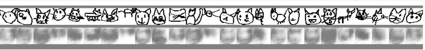
Feeling
- 어제 오전 QnA 세션을 마치기 전에 코치님이 '내일은 노트 내용이 정말 적어서 오후에는 프로젝트 얘기를 해보자~' 라고 하시길래 가벼운 마음으로 하루를 시작했지만,, 실습 코드 이해하고 적는데 정말 오랜 시간이 걸렸다. for문을 저렇게도 쓸 수 있구나 이해한 부분이 재밌었다.
- 뭔가 엄청 큰 무기가 하나씩 주어지는데 내가 그걸 제대로 활용할 수 있을까 하는 걱정이 오늘도 든다. 그만큼 오늘 배운게 되게 멋지고 다양하게 활용해볼 수 있는 흥미로운 기술이라는 말이기도 하다.
B2B SaaS 회사에서 Data Analyst로 일하고 있습니다.