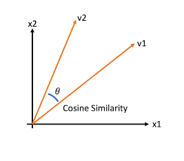
문서와 문서 간의 유사도 비교는 일반적으로 코사인 유사도(Cosine Similarity)를 사용한다. 이는 벡터와 벡터 간의 유사도를 비교할 때 벡터의 크기보다는 벡터의 상호 방향성이 얼마나 유사한지에 기반한다. 즉, 코사인 유사도는 두 벡터 사이에 사잇각을 구해서 얼마나 유사한지 수치로 적용한 것이 된다.
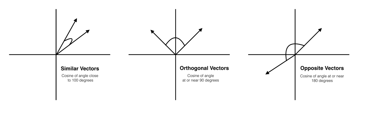
코사인 유사도는 -1 ~ 1 사이의 값을 가진다. 벡터의 각도가 180일때(방향이 완전 다를 경우) -1의 값을 가지며, 값이 90도일 경우 0의 값을 가지게 된다.
문서 유사도 이해하기

0은 관계 없음. 1은 완전히 동일 . -1은 반대방향을 의미한다.
코사인 유사도는 벡터와 벡터 간의 유사도를 비교할 때 벡터의 크기보다는 상호 방향성이 얼마나 유사한지에 기반하며, 유사도 cosθ은 위의 식으로 표현해 볼 수 있다.
간단한 문서에 대해서 서로 간의 문서 유사도를 코사인 유사도 기반으로 구해보자. 먼저 두 개의 넘파이 배열에 대한 코사인 유사도를 구하는 함수를 작성해보겠다.
# 코사인 유사도를 구하는 사용자 함수(551p)
# v1, v2는 좌표값
def cos_simility(v1, v2) :
    dot_product = np.dot(v1, v2)
    l2_norm = (np.sqrt(sum(np.square(v1))) * np.sqrt(sum(np.square(v2))))
    similarity = dot_product / l2_norm

    return similarity


from sklearn.feature_extraction.text import TfidfVectorizer
doc_list = ['if you take the blue pill, the story ends' ,
            'if you take the red pill, you stay in Wonderland',
            'if you take the red pill, I show you how deep the rabbit hole goes']

tfidf_vect = TfidfVectorizer()
feature_vect = tfidf_vect.fit_transform(doc_list)

print(feature_vect.shape)
(3, 18)doc_list로 정의된 3개의 간단한 문서를 TF-IDF 피처 벡터화 시켰다 각 문서별로 18개의 word 피처를 가지고 있는 모습
반환된 행렬은 희소 행렬이므로 앞에서 작성한 cos_similarity() 함수의 인자인 array로 만들기 위해 밀집 행렬로 변환한 뒤 다시 각각을 배열로 변환해야 한다.
# Sparse Matrix(희소행렬)형태를 Dense Matrix(밀집 행렬)로 변환
feature_vect_dense = feature_vect.todense() # toarray()도 가능

# 첫 번째, 두 번째 문서 피처 벡터 추출
vect1 = np.array(feature_vect_dense[0]).reshape(-1,)
vect2 = np.array(feature_vect_dense[1]).reshape(-1,)

# 코사인 유사도
similarity_simple = cos_simility(vect1, vect2 )
print(f"문서 1, 문서 2 Cosine 유사도: {similarity_simple:.3f}")
문서 1, 문서 2 Cosine 유사도: 0.402두 문장 사이의 코사인 유사도는 0.402로 나왔다.
사이킷 런에는 코사인 유사도를 측정하기 위해 API를 제공한다. cosine_similarity() 함수는 두 개의 입력 파라미터를 받는데 첫번째 파라미터는 비교 기준이 되는 문서의 피처 행렬, 두 번째 파라미터는 비교되는 문서의 피처 행렬이다.
이 함수는 희소 행렬, 밀집 행렬 모두가 가능하며, 행렬, 배열도 가능하다.
from sklearn.metrics.pairwise import cosine_similarity

similarity_simple_pair = cosine_similarity(feature_vect[0], feature_vect)
print(similarity_simple_pair)
[[1. 0.40207758 0.40425045]]- 첫번째 값인 1은 비교 기준인 첫번째 문서 자신에 대한 유사도 측정값
- 두번째 값은 첫번째와 두번째 문서의 유사도
- 세번째 값은 첫번째와 세번째 문서의 유사도 값
Opinion Review를 이용한 문서 유사도 측정
데이터, 데이터 불러오기, 피처 벡터화, K-Means는 이전에 해줬던 것과 동일하다.
데이터 불러오기
import numpy as np
import pandas as pd
import glob, os

pd.set_option('display.max_colwidth', 700)

path = r'./OpinosisDataset1.0/OpinosisDataset1.0/topics'

# path로 지정한 디렉토리 밑에 있는 모든 `.data` 파일들의 파일명을 리스트로 취함
all_files = glob.glob(os.path.join(path, "*.data"))
filename_list = []
opinion_text = []

# 개별 파일들의 파일명은 filename_list로 취합
# 개별 파일들의 파일 내용은 DF 로딩 후 다시 string으로 변환하여 opinion_text 리스트로 취합
for file_ in all_files:
    # 개별 파일을 읽어서 DF으로 생성
    df = pd.read_table(file_,index_col=None, header=0,encoding='latin1')

    # 절대 경로로 주어진 파일명을 가공
    # 확장자 제거
    filename_ = file_.split('\\')[-1]
    filename = filename_.split('.')[0]

    filename_list.append(filename)
    opinion_text.append(df.to_string())

    # 파일명 리스트와 파일 내용 리스트를 DataFrame으로 생성
document_df = pd.DataFrame({'filename':filename_list, 'opinion_text':opinion_text})
피처 벡터화
from nltk.stem import WordNetLemmatizer
import nltk
import string

# 단어 원형 추출 함수
lemmar = WordNetLemmatizer()
def LemTokens(tokens):
    return [lemmar.lemmatize(token) for token in tokens]

# 특수 문자 사전 생성: {33: None ...}
# ord(): 아스키 코드 생성
remove_punct_dict = dict((ord(punct), None) for punct in string.punctuation)

# 특수 문자 제거 및 단어 원형 추출
def LemNormalize(text):
    # 텍스트 소문자 변경 후 특수 문자 제거
    text_new = text.lower().translate(remove_punct_dict)

    # 단어 토큰화
    word_tokens = nltk.word_tokenize(text_new)

    # 단어 원형 추출
    return LemTokens(word_tokens)


from sklearn.feature_extraction.text import TfidfVectorizer

tfidf_vect = TfidfVectorizer(stop_words='english' , ngram_range=(1,2),
                             tokenizer = LemNormalize, min_df=0.05, max_df=0.85)

# 피처 벡터화: TF-IDF
feature_vect = tfidf_vect.fit_transform(document_df['opinion_text'])
KMeans-3
from sklearn.cluster import KMeans

# KMeans: 3
km_cluster = KMeans(n_clusters=3, max_iter=10000, random_state=0)
km_cluster.fit(feature_vect)

# cluster 및 중심 좌표 정보
cluster_label = km_cluster.labels_
cluster_centers = km_cluster.cluster_centers_

# cluster 라벨 추가
document_df['cluster_label'] = cluster_label
문서 유사도
from sklearn.metrics.pairwise import cosine_similarity

# cluster_label=2(호텔)인 인덱스
# DataFrame 에서 해당 인덱스를 추출하겠다.
hotel_indexes = document_df[document_df['cluster_label']==2].index
print(f'호텔로 클러스터링 된 문서들의 DataFrame Index : {hotel_indexes}')

# 호텔 군집 중 첫 번째 문서 파일명
comparison_docname = document_df.iloc[hotel_indexes[0]]["filename"]
print("호텔 군집 첫 문서:", comparison_docname)

# 호텔 군집 첫 번째 문서와 호텔 군집 문서 전체간의 코사인 유사도
similarity_pair = cosine_similarity(feature_vect[hotel_indexes[0]] , feature_vect[hotel_indexes])
print(similarity_pair)
호텔로 클러스터링 된 문서들의 DataFrame Index : Int64Index([1, 13, 14, 15, 20, 21, 24, 28, 30, 31, 32, 38, 39, 40, 45, 46], dtype='int64')
호텔 군집 첫 문서: bathroom_bestwestern_hotel_sfo
[[1. 0.0430688 0.05221059 0.06189595 0.05846178 0.06193118
0.03638665 0.11742762 0.38038865 0.32619948 0.51442299 0.11282857
0.13989623 0.1386783 0.09518068 0.07049362]]index를 활용해 호텔 군집 첫 번째 문서, 호텔 군집 문서 전체의 코사인 유사도를 확인하였으며, 직관적으로 확인할 수 있게끔 시각화해보자
import seaborn as sns
import numpy as np
import matplotlib.pyplot as plt

# 첫번째 문서와 타 문서간 유사도가 큰 순으로 정렬한 인덱스를 추출
# 그러나 자기 자신은 제외
sorted_index = similarity_pair.argsort()[:,::-1]
sorted_index = sorted_index[:,1:]

# 유사도가 큰 순서대로 hotel_indexes를 추출하여 재정렬
hotel_sorted_indexes = hotel_indexes[sorted_index.reshape(-1)]

# 유사도가 큰 순으로 유사도 값을 재정렬하되 자기 자신은 제외
hotel_1_sim_value = np.sort(similarity_pair.reshape(-1))[::-1]
hotel_1_sim_value = hotel_1_sim_value[1:]

# 유사도가 큰 순으로 정렬된 인덱스와 유사도 값을 이용해
# 파일명과 유사도 값을 막대그래프 시각화하겠다.
hotel_1_sim_df = pd.DataFrame()
hotel_1_sim_df['filename'] = document_df.iloc[hotel_sorted_indexes]['filename']
hotel_1_sim_df['similarity'] = hotel_1_sim_value

print('가장 유사도가 큰 파일명 및 유사도 :')
print(hotel_1_sim_df)

sns.barplot(x='similarity', y='filename', data=hotel_1_sim_df)
plt.tile(comparison_docname)
가장 유사도가 큰 파일명 및 유사도 :
filename similarity
32 room_holiday_inn_london 0.514423
30 rooms_bestwestern_hotel_sfo 0.380389
31 rooms_swissotel_chicago 0.326199
39 service_holiday_inn_london 0.139896
40 service_swissotel_hotel_chicago 0.138678
28 price_holiday_inn_london 0.117428
38 service_bestwestern_hotel_sfo 0.112829
45 staff_bestwestern_hotel_sfo 0.095181
46 staff_swissotel_chicago 0.070494
21 location_holiday_inn_london 0.061931
15 free_bestwestern_hotel_sfo 0.061896
20 location_bestwestern_hotel_sfo 0.058462
14 food_swissotel_chicago 0.052211
13 food_holiday_inn_london 0.043069
24 parking_bestwestern_hotel_sfo 0.036387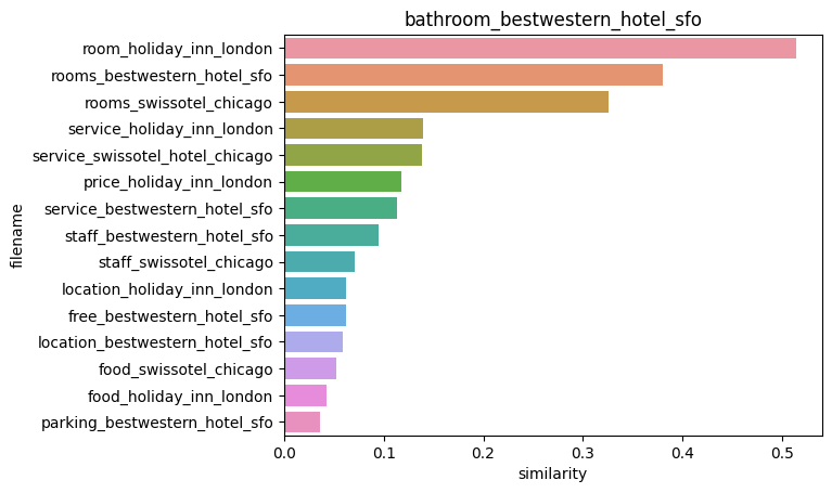
첫번째 문서인 bathroom_bestwestern_hotel_sfo 과 가장 비슷한 문서는 oom_holiday_inn_london 로 약 0.51의 코사인 유사도 값을 보여줬다.