복습 문제
# BOW의 Feature Vectorizer 두가지를 쓰세요
Count, TF_IDF


# 말뭉치 =
corpus
# 어간 추출 =
Stemming
# 표제어 추출
Lemmatization


# 토큰화 두가지
문장 토큰화, 단어 토큰화
sent_tokenize(), word_tokenize()

# BOW 모델은 문서가 가지는 모든 단어를 문맥이나 순서를 무시한다
O


# 텍스트를 피처 벡터화(=워드 임베딩 =Word embedding)의 두가지 방법
1. BOW
2. word2vec


# is, the, a 등 문장을 구성하는 필수 문법 요소이지만 문맥적으로 큰 의미가 없는 단어
stop word


# stemmer.stem('working') 의 출력물을 예측하시오
work


# BOW 형태를 가진 언어 모델의 피처 벡터화는 대부분 ____이다
희소행렬( sparse )


# 희소행렬을 압축해서 저장하는 두가지 방법
COO형식, CSR형식


# 연속된 n개의 단어를 하나의 토큰화 단위로 분리
n-gram


# 카운트 벡터화를 위해 CountVectorizer() 사용하기 전에
# 반드시 텍스트 전처리를 해야한다?
x -- 반드시?
[출제자 답변]
CountVectorizer 클래스에는 소문자 일괄변환, 토큰화, 스톱 워드
필터링등의 텍스트 전처리 기능도 포함하고 있기 때문에 '반드시'는 아니다.


import numpy as np
dense = np.array([[0,1,0,3],
                  [1,2,0,0],
                  [0,0,1,0],
                  [0,2,0,0]])


# COO 형식
data = np.array([1, 3, 1, 2, 1, 2])
row = np.array([0, 0, 1, 1, 2, 3])
col = np.array([1, 3, 0, 1, 2, 1])
from scipy import sparse
sparse.coo_matrix((data, (row, col))).toarray()

# CRS 형식
data = [1, 3, 1, 2, 1, 2]
row_index = np.array([0, 2, 4, 5, 6])
col = [1, 3, 0, 1, 2, 1]
sparse.csr_matrix((data, col, row_index)).toarray()
# [또는]
row_index = np.array([0, 2, 4, 5, 6])
sparse.csr_matrix((data, col, row_index)).toarray()


# 전처리 종류
- 클렌징
- 토큰화
- 스톱워드 제거/필터링/철자 수정
- Stemming/Lemmatization


text = 'I decided, very early on, just to accept life unconditionally.\
        I never expected it to do anything special for me,\
        yet I seemed to accomplish far more than I had ever hoped.\
        Most of the time it just happened to me without my ever seeking it.'

# 위 문장을 전처리 해주세요(특수문자 제거, 토큰화, 스톱워드 제거)

from nltk import word_tokenize, sent_tokenize
import nltk
import re

text1 = re.sub("[^a-zA-Z]", " ", text)
sent_tokenize_sentences = sent_tokenize(text1)
word_tokens = [word_tokenize(sentence) for sentence in sent_tokenize_sentences]

# 영어 stopword
stopwords = nltk.corpus.stopwords.words('english')

# 문장별 단어 토큰화 + stopword 제거
del_stopword_tokens = []

for sentence in word_tokens:
    filtered=[]
    for word in sentence:
        word = word.lower()
        if word not in stopwords:
            filtered.append(word)

    del_stopword_tokens.append(filtered)

print(del_stopword_tokens)
# [추가 답변]
text = text.lower()

# 1. 특수문자 제거
text = re.sub("[^a-zA-Z]", " ", text)

# 2. 단어 토큰화
words = word_tokenize(text)

# 3. 스톱 워드 제거
stopwords = nltk.corpus.stopwords.words('english')
words = [word for word in words if word not in stopwords]
print(words)
DTM
- 문서x 단어행렬 Document Term Matrix
- 특정 문서에 등장하는 특정 단어의 빈도를 나타낸 행렬
- 가로줄(행)에 문서, 세로줄(열)에 단어 배치
- DocumentTermMatrix()
TDM
- 단어x문서 행렬
- TermDocumentMatrix()
IDF
- 역문서 빈도
- Inverse Document Frequency
- log(전체 문서의 수 / term 이 포함된 문서의 수)
TF
- 단어빈도
- Term Frequency
- 특정한 단어가 문서 내에 얼마나 자주 등장하는 지 나타냄
TF-IDF
- TF와 IDF를 곱한 값
- 목적은 다른 문서에 자주 언급되지 않고, 해당문서에서는 자주 언급되는 단어(term, token)에 대해 점수를 높게 부여하는 것이다.
비지도학습 기반 감성 분석
비지도 학습 감성 분석은 Lexicon 이라는 감성사전을 기반으로 하는 것이다. 지도 감성 분석은 데이터 세트가 레이블 값을 가지고 있었지만 많은 감성 분석용 데이터는 이러한 결정된 레이블 값을 가지고 있지 않다. 이런경우에 감성사전(Lexicon)은 유용하게 사용될 수 있다.
감성사전은 긍정 혹은 부정의 감성정도를 의미하는 수치(= 감성 지수)를 가지고 있다.
감성 지수는 단어의 위치, 주변 단어, 문맥, 품사(POS) 등을 참고해 결정된다
WordNet
Synsets은 단어가 가지는 문맥, 시맨틱 정보를 제공하는 WordNet에서의 핵심 개념이다. WordNet을 이용해 Synsets(Sets of cognitive synonyms)를 이해해보자.
먼저 WordNet을 이용하기 위해서는 NLTK를 내려 받아야 하는데 시간이 꽤 걸린다.
import nltk
# NLTK의 모든 데이터 세트와 패키지를 내려 받겠다.
nltk.download('all')
'present' 단어에 Wordnet의 synsets()를 적용해보자
from nltk.corpus import wordnet as wn

synsets = wn.synsets('present')

print(f'synets() 반환 type : {type(synsets)}')
print(f'synets() 반환 값 개수 : {len(synsets)}')
print(f'synets() 반환 값 : {synsets}')
synets() 반환 type : <class 'list'>
synets() 반환 값 개수 : 18
synets() 반환 값 : [Synset('present.n.01'), Synset('present.n.02'), Synset('present.n.03'), Synset('show.v.01'), Synset('present.v.02'), Synset('stage.v.01'), Synset('present.v.04'), Synset('present.v.05'), Synset('award.v.01'), Synset('give.v.08'), Synset('deliver.v.01'), Synset('introduce.v.01'), Synset('portray.v.04'), Synset('confront.v.03'), Synset('present.v.12'), Synset('salute.v.06'), Synset('present.a.01'), Synset('present.a.02')]Synset은 하나의 단어가 가지는 여러 Synset의 객체를 가지는 리스트를 반환한다. 반환값에서 present.n.01 에서 present는 의미 n은 품사(n=명사), 01은 명사의 의미를 구분하는 인덱스다.
synset객체가 가지는 여러가지 속성을 더 살펴볼 수도 있는데. 정의(Definition), 부명제(Lemma), POS(Part of Speech=품사) 등의 시맨틱적 요소를 표현 가능하다 함
for synset in synsets :
    print('##### Synset name : ', synset.name(),'#####')
    print('POS :', synset.lexname())
    print('Definition:', synset.definition())
    print('Lemmas:', synset.lemma_names())
    print()
##### Synset name : present.n.01 #####
POS : noun.time
Definition: the period of time that is happening now; any continuous stretch of time including the moment of speech
Lemmas: ['present', 'nowadays']
##### Synset name : present.n.02 #####
POS : noun.possession
Definition: something presented as a gift
Lemmas: ['present']
##### Synset name : present.n.03 #####
POS : noun.communication
Definition: a verb tense that expresses actions or states at the time of speaking
Lemmas: ['present', 'present_tense']
##### Synset name : show.v.01 #####
POS : verb.perception
Definition: give an exhibition of to an interested audience
Lemmas: ['show', 'demo', 'exhibit', 'present', 'demonstrate']
##### Synset name : present.v.02 #####
POS : verb.communication
Definition: bring forward and present to the mind
Lemmas: ['present', 'represent', 'lay_out']
##### Synset name : stage.v.01 #####
POS : verb.creation
Definition: perform (a play), especially on a stage
Lemmas: ['stage', 'present', 'represent']
##### Synset name : present.v.04 #####
POS : verb.possession
Definition: hand over formally
Lemmas: ['present', 'submit']
##### Synset name : present.v.05 #####
POS : verb.stative
Definition: introduce
Lemmas: ['present', 'pose']
##### Synset name : award.v.01 #####
POS : verb.possession
Definition: give, especially as an honor or reward
Lemmas: ['award', 'present']
##### Synset name : give.v.08 #####
POS : verb.possession
Definition: give as a present; make a gift of
Lemmas: ['give', 'gift', 'present']
##### Synset name : deliver.v.01 #####
POS : verb.communication
Definition: deliver (a speech, oration, or idea)
Lemmas: ['deliver', 'present']
...
이하 생략[ present.n.01, present.n.02 ]는 같은 명사이지만 서로 다른 의미를 가지고 있다는 걸을 보여준다.
WordNet은 어휘 간의 관계를 유사도로 나타내줄 수도 있는데, path_similarity 메서드로 확인 가능하다.
# synset 객체를 단어별로 생성
tree = wn.synset('tree.n.01')
lion = wn.synset('lion.n.01')
tiger = wn.synset('tiger.n.02')
cat = wn.synset('cat.n.01')
dog = wn.synset('dog.n.01')

# 여러 객체를 하나의 리스트로 생성
entities = [tree , lion , tiger , cat , dog]

# 각 객체별 다른 객체와의 유사도 측정 후 담아줄 빈 리스트
similarities = []

# 각 객체의 이름 리스트
entity_names = [ entity.name().split('.')[0] for entity in entities]

# 단어별 synset을 반복하면서 다른 단어의 synset과 유사도를 측정
for enity in entities :
    similarity = [round(enity.path_similarity(compared_entity), 2)
                 for compared_entity in entities]
    similarities.append(similarity)

similarities
[[1.0, 0.07, 0.07, 0.08, 0.12],
[0.07, 1.0, 0.33, 0.25, 0.17],
[0.07, 0.33, 1.0, 0.25, 0.17],
[0.08, 0.25, 0.25, 1.0, 0.2],
[0.12, 0.17, 0.17, 0.2, 1.0]]# 개별 단어별 synset과 다른 단어의 synset과의 유사도를 DataFrame형태로 저장
similarity_df = pd.DataFrame(similarities, columns=entity_names, index=entity_names)
similarity_df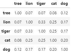
-tree 는 lion과 tiger와 유사도가 낮고 그나마 dog와 유사도가 높다.
-cat은 tree와 유사도가 가장 낮았고 lion과는 유사도가 높다.
SentiWordnet은 WordNet의 Synset과 유사한 Senti_Synset클래스를 가지고 있다. 리스트 형태로 반환한다.
import nltk
from nltk.corpus import sentiwordnet as swn

senti_synsets = list(swn.senti_synsets('slow'))

print(f'senti_synsets() 반환 type : {type(senti_synsets)}')
print(f'senti_synsets() 반환 값 개수 : {len(senti_synsets)}')
print(f'senti_synsets() 반환값 : {senti_synsets}')
senti_synsets() 반환 type : <class 'list'>
senti_synsets() 반환 값 개수 : 11
senti_synsets() 반환값 : [SentiSynset('decelerate.v.01'), SentiSynset('slow.v.02'), SentiSynset('slow.v.03'), SentiSynset('slow.a.01'), SentiSynset('slow.a.02'), SentiSynset('dense.s.04'), SentiSynset('slow.a.04'), SentiSynset('boring.s.01'), SentiSynset('dull.s.08'), SentiSynset('slowly.r.01'), SentiSynset('behind.r.03')]SentiSynser 객체는 단어의 감성을 나타내는 감성 지수(긍정/부정)와 객관성 지수를 가지고 있다.
감성지수와 객관성 지수는 비례 개념으로, 감성지수가 0이라면 객관성지수는 1이 된다. father(아빠)-fabulous(아주멋진) 사이의 감성지수와 객관성 지수를 구해보자
import nltk
from nltk.corpus import sentiwordnet as swn

father = swn.senti_synset('father.n.01')
print('father 긍정 감성 지수: ', father.pos_score())
print('father 부정 감성 지수: ', father.neg_score())
print('father 객관성 지수: ', father.obj_score())
print()

fabulous = swn.senti_synset('fabulous.a.01')
print('fabulous 긍정 감성 지수: ',fabulous.pos_score())
print('fabulous 부정 감성 지수: ',fabulous.neg_score())
print('fabulous 객관성 지수: ', fabulous.obj_score())
father 긍정 감성 지수: 0.0
father 부정 감성 지수: 0.0
father 객관성 지수: 1.0
fabulous 긍정 감성 지수: 0.875
fabulous 부정 감성 지수: 0.125
fabulous 객관성 지수: 0.0SentiWordNet 감성 분석
SentiWordNet을 이용해 감성 분석을 수행하는 대략적인 순서는 아래와 같다.
1. 문서(Document)를 문장(Sentence) 단위로 분해
2. 다시 문장을 단어(Word) 단위로 토큰화하고 품사 태깅
3. 품사 태깅된 단어를 기반으로 synset 객체와 senti_synset 객체를 생성
4. Senti_synset에서 긍정 감성/부정 감성 지수를 구하고 이를 모두 합산해 특정 임계치 값 이상일 때 긍정감성으로, 그렇지 않을 때는 부정 감성으로 결정
품사 태깅 사용자 함수
from nltk.corpus import wordnet as wn

def penn_to_wn(tag):
    # 형용사
    if tag.startswith('J'):
        return wn.ADJ

    # 명사
    elif tag.startswith('N'):
        return wn.NOUN

    # 부사
    elif tag.startswith('R'):
        return wn.ADV
    # 동사
    elif tag.startswith('V'):
        return wn.VERB
    return
긍정/부정 예측 사용자 함수
문장 → 단어토큰 → 품사 태깅
후 SentiSynset 클래스를 생성하여 Polarity Score를 합산하는 함수를 생성하기로 한다. 각 단어의 긍정/부정 감성지수를 모두 합한 총 감성 지수가 0 이상일 경우 긍정감성이라고 예측한다.
from nltk.stem import WordNetLemmatizer
from nltk.corpus import sentiwordnet as swn
from nltk import sent_tokenize, word_tokenize, pos_tag

def swn_polarity(text):
    # 감성 지수 초기화
    sentiment = 0.0
    tokens_count = 0

    # 어근 추출 객체
    lemmatizer = WordNetLemmatizer()

    # 문장 토큰화
    raw_sentences = sent_tokenize(text)

    # 분해된 문장별로 단어 토큰 -> 품사 태깅 후에 SentiSynset 생성 -> 감성 지수 합산
    for raw_sentence in raw_sentences:
        # 각 문장별 단어 토큰화 후 품사 태깅 문장 추출 (단어와 품사 생성)
        tagged_sentence = pos_tag(word_tokenize(raw_sentence))

        for word , tag in tagged_sentence:
            # WordNet 기반 품사 태깅
            wn_tag = penn_to_wn(tag)
            if wn_tag not in (wn.NOUN , wn.ADJ, wn.ADV):
                continue

            # 어근 추출
            lemma = lemmatizer.lemmatize(word, pos=wn_tag)
            if not lemma:
                continue

            # 어근 추출한 단어, WordNet 기반 품사 태깅을 입력해 Synset 객체 생성
            synsets = wn.synsets(lemma , pos=wn_tag)

            if not synsets:
                continue

            # 생성된 synset 객체의 첫 번째 의미 사용
            # 같은 품사여도 여러 의미 존재할 수 있기 때문에
            synset = synsets[0]

            # 이용해서 SentiSynset 객체 생성
            swn_synset = swn.senti_synset(synset.name())

            # 긍정 감성 지수 - 부정 감성 지수로 감성 지수 계산
            sentiment += (swn_synset.pos_score() - swn_synset.neg_score())
            tokens_count += 1

    if not tokens_count:
        return 0

    # 총 score가 0 이상일 경우 긍정(Positive) 1, 그렇지 않을 경우 부정(Negative) 0 반환
    if sentiment >= 0 :
        return 1

    return 0
이렇게 생성한 함수는 IMDB 감상평의 개별 문서에 적용해 긍정 및 부정 감성을 예측할 수 있게 한다.
review_df['preds'] = review_df['review'].apply(lambda x : swn_polarity(x))텍스트 별로 '긍정/부정 예측 사용자 함수'를 호출하기 때문에 수행시간이 꽤 길다.
review_df['preds']가 만들어졌다면, 사용 목적에 맞게 나눠주자
y_target = review_df['sentiment'].values
preds = review_df['preds'].values
이제 SentiWordNet의 '감성 분석 예측'의 성능을 살펴보려 한다. 이전에 만들어 사용했던 '사용자 평가 지표' 함수를 이용해보겠다.
from sklearn.metrics import accuracy_score, precision_score, recall_score, confusion_matrix
from sklearn.metrics import f1_score, roc_auc_score

def get_clf_eval(y_test, pred=None, pred_proba_po=None):
    confusion = confusion_matrix(y_test, pred)
    accuracy = accuracy_score(y_test, pred)
    precision = precision_score(y_test, pred)
    recall = recall_score(y_test, pred)
    f1 = f1_score(y_test, pred)


    print("오차 행렬")
    print(confusion)
    print(f"정확도: {accuracy:.4f}, 정밀도: {precision:.4f}, 재현율: {recall:.4f}, F1: {f1:.4f}")


get_clf_eval(y_target, pred=preds)
오차 행렬
[[7668 4832]
[3636 8864]]
정확도: 0.6613, 정밀도: 0.6472, 재현율: 0.7091, F1: 0.6767정확도 : 약 0.66
정밀도 : 약 0.65
재현율 : 약 0.70정도의 수치가 나왔다. 예측 정확도가 약 0.8936 정도 나왔던 지도학습에 비했을때 확실히 낮은 수치임을 알 수 있다.
VADER 감성 분석
SNS의 감성 분석 용도로 만들어진 룰 기반의 Lexicon 이다.
먼저 SentimentintensityAnalyzer 클래스를 이용해 객체를 생성한 뒤 문서별로 polarity_scores() 메서드를 호출하여 감성점수를 구하고, 해당 문서의 감성 점수가 특정 임계값 이상이면긍정, 그렇지 않으면 부정으로 판단한다.
from nltk.sentiment.vader import SentimentIntensityAnalyzer
senti_analyzer = SentimentIntensityAnalyzer()
senti_scores = senti_analyzer.polarity_scores(review_df['review'][0])
print(senti_scores){'neg': 0.13, 'neu': 0.743, 'pos': 0.127, 'compound': -0.7943}neg는 중립적인 감성지수 / POS는 긍정 감성 / compound는- 1 ~ 1 사이의 값을 가지며 보통 0.1 이상이면 긍정으로 판단한다.
임계치별 긍정/부정 예측 함수
from nltk.sentiment.vader import SentimentIntensityAnalyzer
def vader_polarity(review, threshold = 0.1):
# VADER 객체로 감성 지수 산출
analyzer = SentimentIntensityAnalyzer()
scores = analyzer.polarity_scores(review)
# compound 값에 기반해
# threshold 보다 크거나 같으면 1, 그렇지 않으면 0 을 반환하도록 한다.
agg_score = scores['compound']
final_sentiment = 1 if agg_score >= threshold else 0
return final_sentiment아래 코드 역시 텍스트별로 사용자 함수(vader_polarity)를 호출하기 때문에 꽤 오랜 수행시간이 걸린다.
# 각 문서별로 긍정/부정 예측
review_df['vader_preds'] = review_df['review'].apply( lambda x : vader_polarity(x, 0.1) )그 후 각 문서별로 긍정/부정 예측을 하면
y_target = review_df['sentiment'].values
vader_preds = review_df['vader_preds'].values
get_clf_eval(y_target, pred=vader_preds)오차 행렬
[[ 6747 5753]
[ 1858 10642]]
정확도: 0.6956, 정밀도: 0.6491, 재현율: 0.8514, F1: 0.7366이전에 한 결과가
정확도 : 약 0.66
정밀도 : 약 0.65
재현율 : 약 0.70였는데 정확도와 재현율이 많이 오른 대신 정밀도가 조금 떨어진 모습이다.
문서 군집화
문서 군집화(Document Clustering)는 비슷한 텍스트 구성의 문서를 군집화(Clustering) 하는 방법이다. 텍스트 분류와 비슷하지만 문서 군집화는 학습 데이터 세트가 필요없는 비지도 학습을 기반이다.
Opinin Review를 이용한 실습
Opinion Review 데이터를 사용할 것이다.
import numpy as np
import pandas as pd
import glob, os

pd.set_option('display.max_colwidth', 700)

path = r'./OpinosisDataset1.0/OpinosisDataset1.0/topics'

# path로 지정한 디렉토리 밑에 있는 모든 `.data` 파일들의 파일명을 리스트로 취함
all_files = glob.glob(os.path.join(path, "*.data"))
filename_list = []
opinion_text = []

opinion_text
[" , and is very, very accurate .\n0 but for the most part, we find that the Garmin software provides accurate directions, whereever we intend to go .\n1 This function is not accurate if you don't leave it in battery mode say, when you stop at the Cracker Barrell for lunch and to play one of those trangle games with the tees .\n2 It provides immediate alternatives if the route from the online map program was inaccurate or blocked by an obstacle .\n3 I've used other GPS units, as well as GPS built into cars and to this day NOTHING beats the accuracy of a Garmin GPS .\n4 It got me from point A to point B with 100% accuracy everytime .\n5 It has yet to disappoint, getting me everywhere with 100% accuracy .\n6 0 out of 5 stars Honest, accurate review, , PLEASE READ !\n7
... 이하 생략# 파일명 리스트와 파일 내용 리스트를 DataFrame으로 생성
document_df = pd.DataFrame({'filename':filename_list, 'opinion_text':opinion_text})
document_df[:3]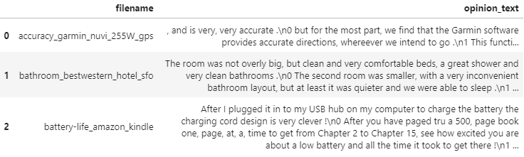
document_df.count()filename 51
opinion_text 51
cluster_label 51
dtype: int64해당 데이터 세트는 51개의 텍스트 파일로 구성되어 있고, 각 파일명과 파일 내용을 DataFrame으로 생성하였다.
문서의 유형은 크게 보자면 전자제품, 자동차, 호텔로 되어있다. 전자제품은 다시 내비게이션, 아이팟, 킨들, 랩톱 콤퓨터 등과 같은 세부 요소로 나뉜다.
전반적으로 군집화된 결과를 살펴보면 군집 개수가 약간 많게 설정이 된 듯 잘 못 분류된 것들이 군집에 섞여있는 모습이였다.
피처 벡터화
tokenizer 함수
from nltk.stem import WordNetLemmatizer
import nltk
import string

# 단어 원형 추출 함수
lemmar = WordNetLemmatizer()
def LemTokens(tokens):
    return [lemmar.lemmatize(token) for token in tokens]

# 특수 문자 사전 생성: {33: None ...}
# ord(): 아스키 코드 생성
remove_punct_dict = dict((ord(punct), None) for punct in string.punctuation)

# 특수 문자 제거 및 단어 원형 추출
def LemNormalize(text):
    # 텍스트 소문자 변경 후 특수 문자 제거
    text_new = text.lower().translate(remove_punct_dict)
    # 단어 토큰화
    word_tokens = nltk.word_tokenize(text_new)
    # 단어 원형 추출
return LemTokens(word_tokens) string.punctuation은 느낌표, 물음표, 더하기 등의 문자dict((ord(punct), None) for punct in string.punctuation)로 해당 문자 사전을 생성하였다.text.lower().translate(remove_punct_dict)로 문자 사전에 따라 None으로 변환하였고, 그 후 단어 토큰화 후에 토큰별로 원형을 추출한다.
from sklearn.feature_extraction.text import TfidfVectorizer

tfidf_vect = TfidfVectorizer(tokenizer=LemNormalize, stop_words='english', ngram_range=(1,2), min_df=0.05, max_df=0.85 )

# opinion_text 칼럼 값으로 feature vectorization 수행
feature_vect = tfidf_vect.fit_transform(document_df['opinion_text'])
피처 벡터화로 TF-IDF를 사용했다. tokenizer로 앞서 만든 사용자 함수를 적용
→ 피처 벡터화에서 Stemmer, Lemmatize는 tokenizer로 수행한다.
K-Means
군집화 기법으로 K-Means를 적용할 것이다. 먼저 5개의 중심(Centriod) 기반으로 어떻게 군집화되는지 확인해보려 한다.
최대반복횟수(max_iter)는 10000으로 설정하고, KMeans를 수행한 뒤에 군집의 Label 값과 중심별로 할당된 데이터 세트의 좌표 값을 구해볼 것이다.
from sklearn.cluster import KMeans

# 5개의 집합으로 군집화 수행
km_cluster = KMeans(n_clusters=5, max_iter=10000, random_state=0)

km_cluster.fit(feature_vect)
cluster_label = km_cluster.labels_
cluster_centers = km_cluster.cluster_centers_

document_df['cluster_label'] = cluster_label
document_df[:3]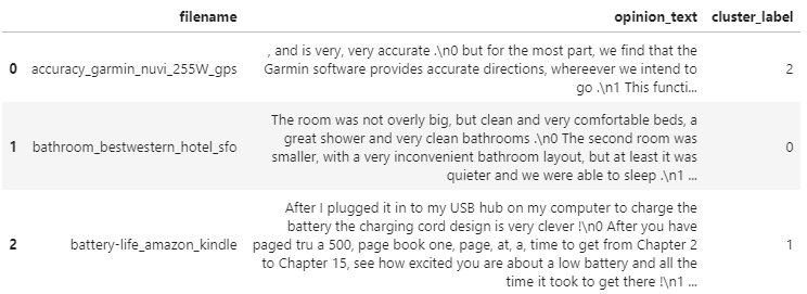
판다스 DataFrame의 sort_values(by=정렬칼럼명)을 수행하면 인자로 입력된 '정렬칼럼명'으로 데이터를 정렬할 수 있다.
document_df[document_df['cluster_label']==0].sort_values(by='filename')
document_df[document_df['cluster_label']==1].sort_values(by='filename')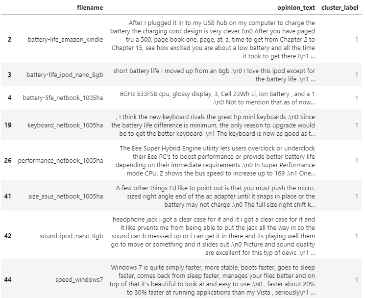
0번 군집은 호텔에 대한 리뷰로, 1번 군집은 킨들, 아이팟, 넷북 등 전자기기에 대한 리뷰로 군집화 되어있다. 이외에도 2번 군집은 토요타, 혼다 등 자동차에 대한 리뷰, 3번 군집은 킨들에 대한 리뷰, 4번 군집은 네이게이션에 대한 리뷰로 군집화 되어 있는 것을 확인 할 수 있다.
from sklearn.cluster import KMeans

# 3개의 집합으로 군집화
km_cluster = KMeans(n_clusters=3, max_iter=10000, random_state=0)
km_cluster.fit(feature_vect)
cluster_label = km_cluster.labels_
n_clusters를 5에서 3으로 낮춰주었다
# 소속 클러스털르 cluster_label 칼럼으로 할당하고 cluster_label 값으로 정렬
document_df['cluster_label'] = cluster_label
document_df.sort_values(by='cluster_label')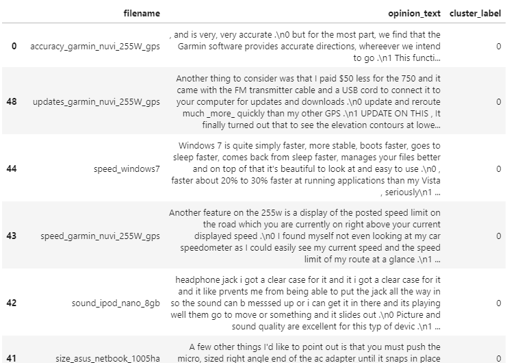
document_df[document_df['cluster_label']==0].sort_values(by='filename')
document_df[document_df['cluster_label']==1].sort_values(by='filename')
document_df[document_df['cluster_label']==2].sort_values(by='filename')
결과를 확인해보면
0번 군집 : 포터블 전자기기 리뷰
1번 군집 : 자동차 리뷰
2번 군집 : 호텔리뷰
로만 군집이 잘 구성된 모습이였다.
군집별 핵심 단어 추출하기
각 군집에 속한 문서는 핵심 단어를 주축으로 군집화 되어 있을 것이다. 이번에는 각 군집을 구성하는 핵심 단어가 어떤 것이 있는지 확인해 보려 한다.
이전에 공부했 듯 KMeans의 cluster_centers_ 속성은 군집별 피처의 중심점 좌표를 가지고 있다. 이는 배열값으로 제공되며 행은 개별 군집을, 열은 개별 피처를 의미한다.
cluster_centers = km_cluster.cluster_centers_
print(f'cluster_centers shaper : {cluster_centers.shape}')
print(cluster_centers)
cluster_centers shaper : (3, 4611)
[[0.01005322 0. 0. ... 0.00706287 0. 0. ]
[0. 0.00092551 0. ... 0. 0. 0. ]
[0. 0.00099499 0.00174637 ... 0. 0.00183397 0.00144581]](3, 4611)는 배열이다. 이는 군집이 3개, word 피처가 4611개로 구성되어 있음을 의미한다. 각 행의 배열 값은 군집 내의 피처가 개별 중심과 얼마나 가까운가를 상대 값으로 나타낸 것이다.
0에서 1까지의 값을 가질 수 있으며 1에 가까울 수록 중심과 가까운 값을 의미한다.
이제 이를 이용해 각 군집별 핵심단어를 찾아보려 한다. cluster_centers_ 속성은 numpy의 ndarray이고, 이는 argsort()[:,::-1]를 이용하면 배열 내 값이 큰 순으로 정렬된 위치 인덱스 값을 반환받을 수 있다는 것이다.
※ 유의할 점은 큰 값으로 정렬된 값을 반환하는 게 아니라 큰 값을 가진 배열 내 위치 인덱스 값을 반환한다는 것이다.
군집별 top n개의 핵심단어, 그 단어의 중심 위치 상대값, 대상 파일명을 반환하는 사용자 정의 함수를 작성해보자
def get_cluster_details(cluster_model, cluster_data, cluster_nums, feature_names, top_n_features=10):

    # 핵심 단어 등 정보를 담을 딕셔너리 생성
    cluster_details = {}

    # word 피처 중심과의 거리 내림차순 정렬시 값들의 index 반환
    center_info = cluster_model.cluster_centers_        # 군집 중심 정보
    center_descend_ind = center_info.argsort()[:, ::-1] # 행별(군집별)로 역순 정렬

    # 군집별 정보 담기
    for i in range(cluster_nums):
        # 군집별 정보를 담을 데이터 초기화
        cluster_details[i] = {} # 사전 안에 사전

        # 각 군집에 속하는 파일명
        filenames = cluster_data[cluster_data["cluster_label"] == i]["filename"]
        filenames = filenames.values.tolist()

        # 군집별 중심 정보
        top_feature_values = center_info[i, :top_n_features].tolist()

        # 군집별 핵심 단어 피처명
        top_feature_indexes = center_descend_ind[i, :top_n_features]
        top_features = [feature_names[ind] for ind in top_feature_indexes]

        # 각 군집별 정보 사전에 담기
        cluster_details[i]["cluster"] = i                              # i번째 군집
        cluster_details[i]["top_features"] = top_features              # 군집별 핵심 단어
        cluster_details[i]["top_feature_values"] = top_feature_values  # 군집별 중심 정보
        cluster_details[i]["filenames"] = filenames                    # 군집 속 파일명

    return cluster_details
위이 사용자 정의 함수를 호출하면 dictionary를 원소로 가지는 리스트인 cluster_details를 반환한다. 여기에는 개별 군집번호, 핵심단어, 핵심단어의 중심위치 상대값, 파일명 속성 값 정보가 있는데 이를 조금 더 보기 좋게 표현하기 위해 별도의 사용자 함수를 만들어보자.
def print_cluster_details(cluster_details) :
    for cluster_num, cluster_detail in cluster_details.items() :
        print(f'#### Cluster {cluster_num}')
        print(f'Top features : {cluster_detail["top_features"]}')
        print(f'Reviews 파일명 : {cluster_detail["filenames"][:7]}')
        print("=="*15)
이제 위에서 생성한 함수들을 호출해 추출해보려 한다.
feature_names = tfidf_vect.get_feature_names()
cluster_details = get_cluster_details(cluster_model=km_cluster, cluster_data=document_df,
                                     feature_names=feature_names, cluster_nums=3, top_n_features=10)
print_cluster_details(cluster_details)
#### Cluster 0
Top features : ['screen', 'battery', 'keyboard', 'battery life', 'life', 'kindle', 'direction', 'video', 'size', 'voice']
Reviews 파일명 : ['accuracy_garmin_nuvi_255W_gps', 'battery-life_amazon_kindle', 'battery-life_ipod_nano_8gb', 'battery-life_netbook_1005ha', 'buttons_amazon_kindle', 'directions_garmin_nuvi_255W_gps', 'display_garmin_nuvi_255W_gps']
==============================
#### Cluster 1
Top features : ['interior', 'seat', 'mileage', 'comfortable', 'gas', 'gas mileage', 'transmission', 'car', 'performance', 'quality']
Reviews 파일명 : ['comfort_honda_accord_2008', 'comfort_toyota_camry_2007', 'gas_mileage_toyota_camry_2007', 'interior_honda_accord_2008', 'interior_toyota_camry_2007', 'mileage_honda_accord_2008', 'performance_honda_accord_2008']
==============================
#### Cluster 2
Top features : ['room', 'hotel', 'service', 'staff', 'food', 'location', 'bathroom', 'clean', 'price', 'parking']
Reviews 파일명 : ['bathroom_bestwestern_hotel_sfo', 'food_holiday_inn_london', 'food_swissotel_chicago', 'free_bestwestern_hotel_sfo', 'location_bestwestern_hotel_sfo', 'location_holiday_inn_london', 'parking_bestwestern_hotel_sfo']
==============================포터블 전자제품 리뷰 군집인 0번 군집만 보자면 'screen, battery, battery life' 등과 같은 단어들이 핵심 단어로 군집화 되어있다는 걸 확인할 수 있었다.