[ Attention ] bahdanau, luong review

d4r6j·2023년 10월 3일

nlp-paper

목록 보기

1/8

Analysis code : Attention

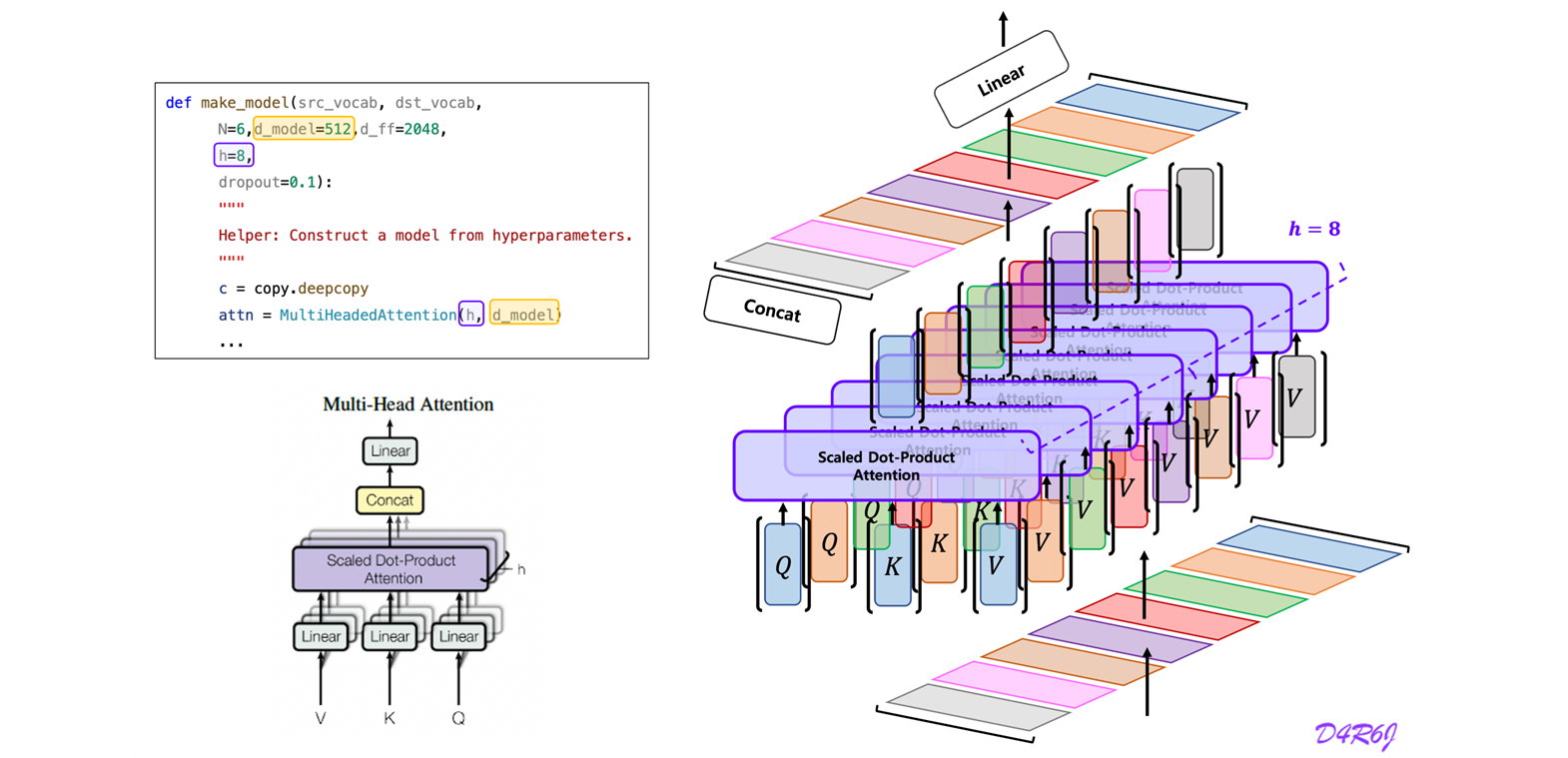
# 1. Do all the linear projections in batch from d_model -> h, x, d_x
query, key, value = \
    [lin(x).view(nbatches, -1, self.h, self.d_k).transpose(1, 2)
        for lin, x in zip(self.linears, (query, key, value))]

# 2. Apply attention on all the projected vectors in batch.
x, self.attn = attention(query,
                            key,
                            value,
                            mask=mask,
                            dropout=self.dropout)

# 3. "Concat" using a view and apply a final linear.
x = x.transpose(1, 2).contiguous().view(nbatches,
                                        -1,
                                        self.h * self.d_k)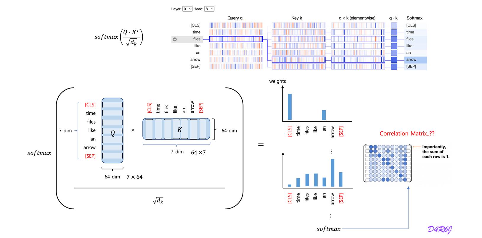

def attention(query: torch.Tensor,
              key: torch.Tensor,
              value: torch.Tensor,
              mask=None,
              dropout=None) -> tuple:
    "Compute 'Scaled Dot Product Attention"
    d_k = query.size(-1)
    scores = torch.matmul(query, key.transpose(-2, -1)) / math.sqrt(d_k)

    if mask is not None:
        scores = scores.masked_fill(mask == 0, -1e9)
    p_attn = F.softmax(scores, dim=-1)

    if dropout is not None:
        p_attn = dropout(p_attn)

    return torch.matmul(p_attn, value), p_attn

What is the "Attention"? : bahdanau, luong

1. Prerequisite

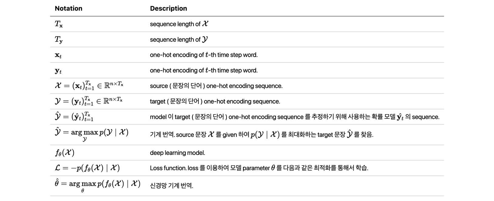
Notation

성능 검증
```
정답 : "I was written by human"
생성 : "I was genereated by Artifical Intelligence"
```
- BLEU (Bilingual Evaluation Understudy)
  - 생성된 문장의 단어가 정답 문장에 얼마나 포함되어 있는 지를 측정하기 위해서 만든 metric.
  - Generated Sentence 의 단어가 Reference Sentence 에 포함되는 정도.
  - 정확도를 요하는 task, 번역 모델에서는 좀 더 정확하게 생성해야 하는 것이 중요하기 때문에 BLUE score.
  - (정답 문장과 생성 문장이 겹치는 단어) / 생성 문장 길이 = 3/6
  - $\frac{TP}{TP + FP}$ (Precision $\rightarrow$ Positive Predictive Value)
- ROUGE (Recall-Oriented Understudy for Gisting Evaluation)
  - 정답 문장의 단어가 생성된 문장에 포함되는 정도를 보기 위한 척도.
  - Reference Sentence 의 단어가 Generated Sentence 에 포함되는 정도.
  - 요약 모델에서는 정확한 정답 보다는 얼마나 겹치느냐가에 좀 더 focus 를 주는 정도.
  - (정답 문장과 생성 문장이 겹치는 단어) / 정답 문장 길이 = 3/7
  - $\frac{TP}{TP + FN}$ (Recall $\rightarrow$ True Positive Rate)
- Perplexity (당혹감, 당혹스러운)
  - 정답 문장의 단어가 생성된 문장에 포함되는 정도를 보기 위한 척도.
  - 텍스트 생성시 헷갈리는 정도로 이해. 언어 모델의 분기 계수 (Branching Factor)
  - 이전 단어로 다음 단어를 예측할 때 몇 개의 단어 후보를 고려하는지를 의미한다. 따라서 낮을 수록 모델의 성능이 우수하다고 평가.
  - 테스트 데이터셋이 충분히 신뢰도가 높을 때 (질적으로, 양적으로 많을 때) 만 적용.
  - 같은 테스트 데이터 셋에서 언어 모델간의 PPL 값을 비교하면 우수한 성능인지 비교 가능.
  - Sequence : 문장은 어순을 고려 (순서를 고려) 하여 여러 단어로 이루어진 Word Sequence.

PPL(W) = P(w_1, w_2, w_3, \cdots, w_N)^{-\frac{1}{N}}=\sqrt[N]{\frac{1}{P(w_1, w_2, w_3, \cdots, w_N)}}

* 문장의 확률에 chain rule 을 적용하면

PPL(W) = \sqrt[N]{\frac{1}{P(w_1, w_2, w_3, \cdots, w_N)}} = \sqrt[N]{\frac{1}{\Pi^{N}_{i=1} P(w_i|w_1, w_2, w_3, \cdots, w_{i-1})}}

2. Machine Translation

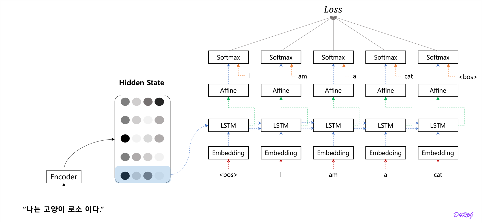
Attention mechanism 이전의 기계번역 모델의 기본 구조.
RNN Cell 을 이용해서 encoder, decoder 로 구성, 맨 마지막 화살표가 encoder 의 hidden state.
encoder 전체의 문장 정보를 다 학습하여진 함축 되어 있는 하나의 vector
이 hidden state vector 를 활용해서 decoder 는 문장을 생성.

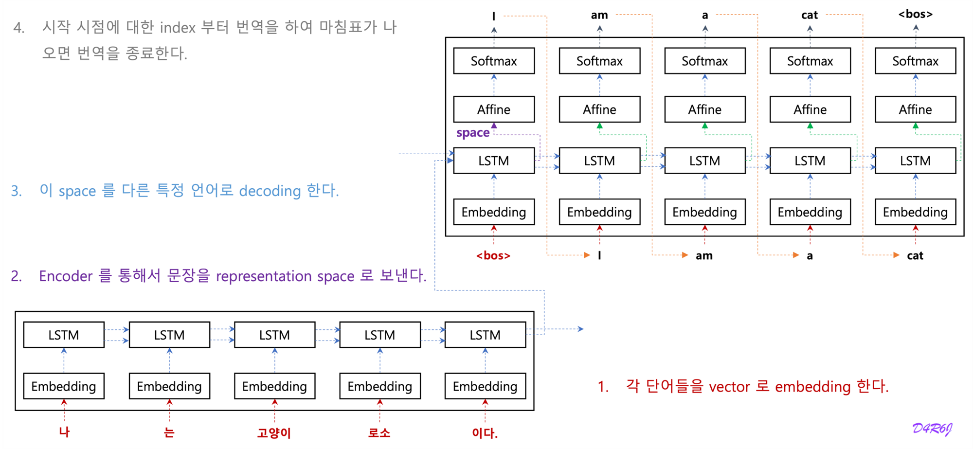
3. Encoder-Decoder model

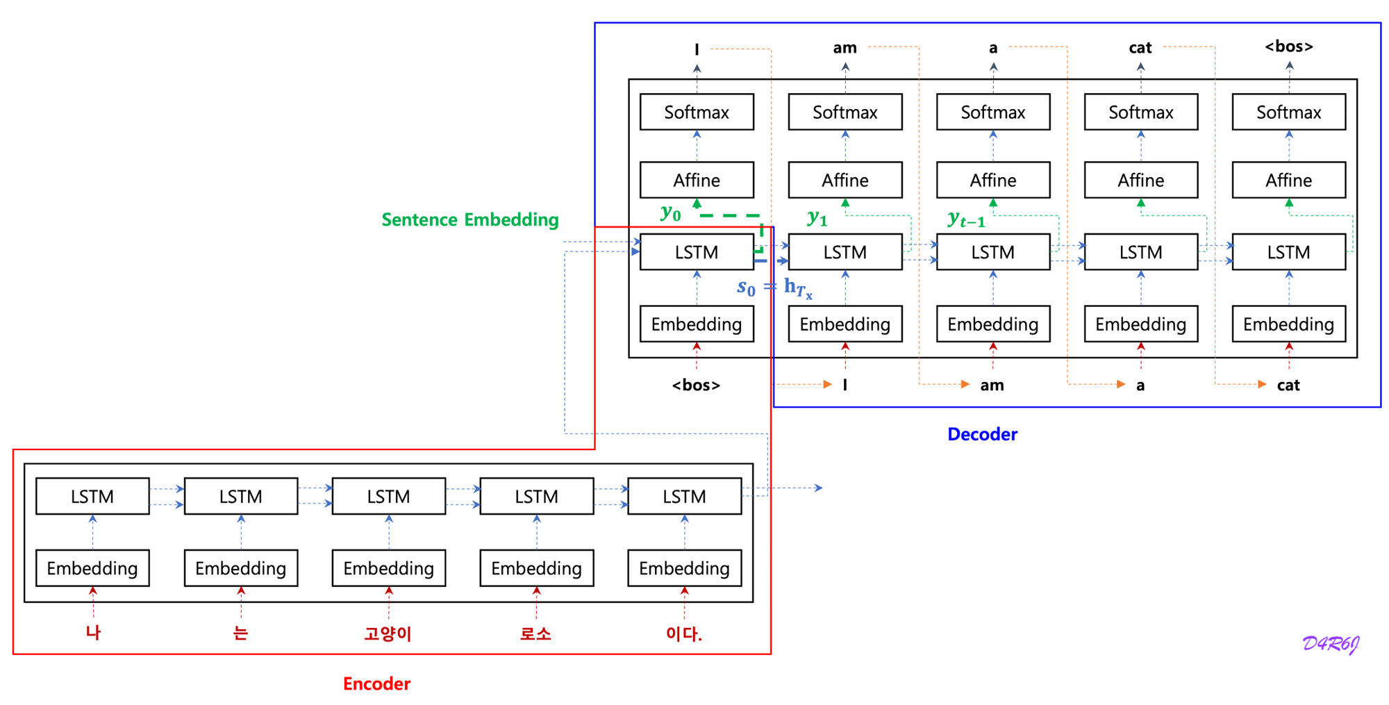
\hat{\mathbf{y}}_t = p(\hat{\mathbf{y}}_t|\hat{\mathbf{y}}_0, \cdots, \hat{\mathbf{y}}_{t-1}, \mathcal{X}) = {\rm Softmax (W_y s_t + b)}

s_t = {\rm tanh(W_{ys}y_{t-1} + W_{ss}s_{t-1} + b_s) \quad where \quad \mathbf{y}_0}={\rm Enc(\mathcal{X}), \; s_0 = \mathbf{h}_{T_x}}

Notation
- $\mathbf{y}_0$ 는 인코더가 최종적으로 생성한 문장 embedding.
  - decoder RNN 은 입력으로 이전 time step 의 encoder output 을 받는 구조.
- $\mathbf{s}_t$ 는 $t$ 번째 time step 의 decoder RNN Hidden State Vetor
- ${\rm h}_{T_x}$ 는 마지막 time step 의 encoder RNN Hidden State Vector
- ${\rm s}_0$ 는 decoder 의 첫 번째 time step 의 Hidden State Vector
Sentence Embedding problem.
- long term dependency.
  - RNN 구조 특성상, 현재 time step 과 멀어지면 멀어질수록, 해당 정보에 대한 손실이 커진다는 문제.
- vector of fixed length.
  - Encoder 가 시계열 데이터를 encoding 하고 그 정보를 Decoder 로 전달 하는데, 이때 Encoder 의 출력은 '고정 길이의 벡터'.
  - '고정 길이의 벡터' 에 문제가 있다. 입력 문장의 길이에 관계 없이 (아무리 길어도), 항상 같은 길이의 벡터로 변환한다는 뜻.
  - 문장이 길어질수록 더 많은 정보가 고정된 길이로 압축하므로, 필요한 정보가 vector 에 모두 담기지 못하는 정보 손실의 문제.

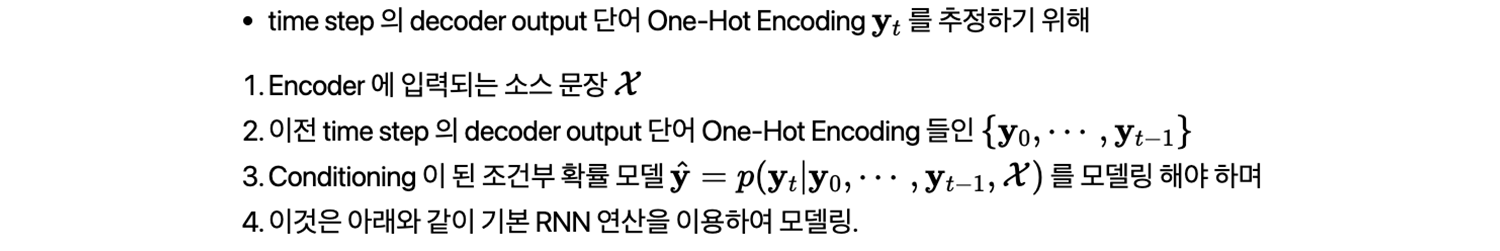
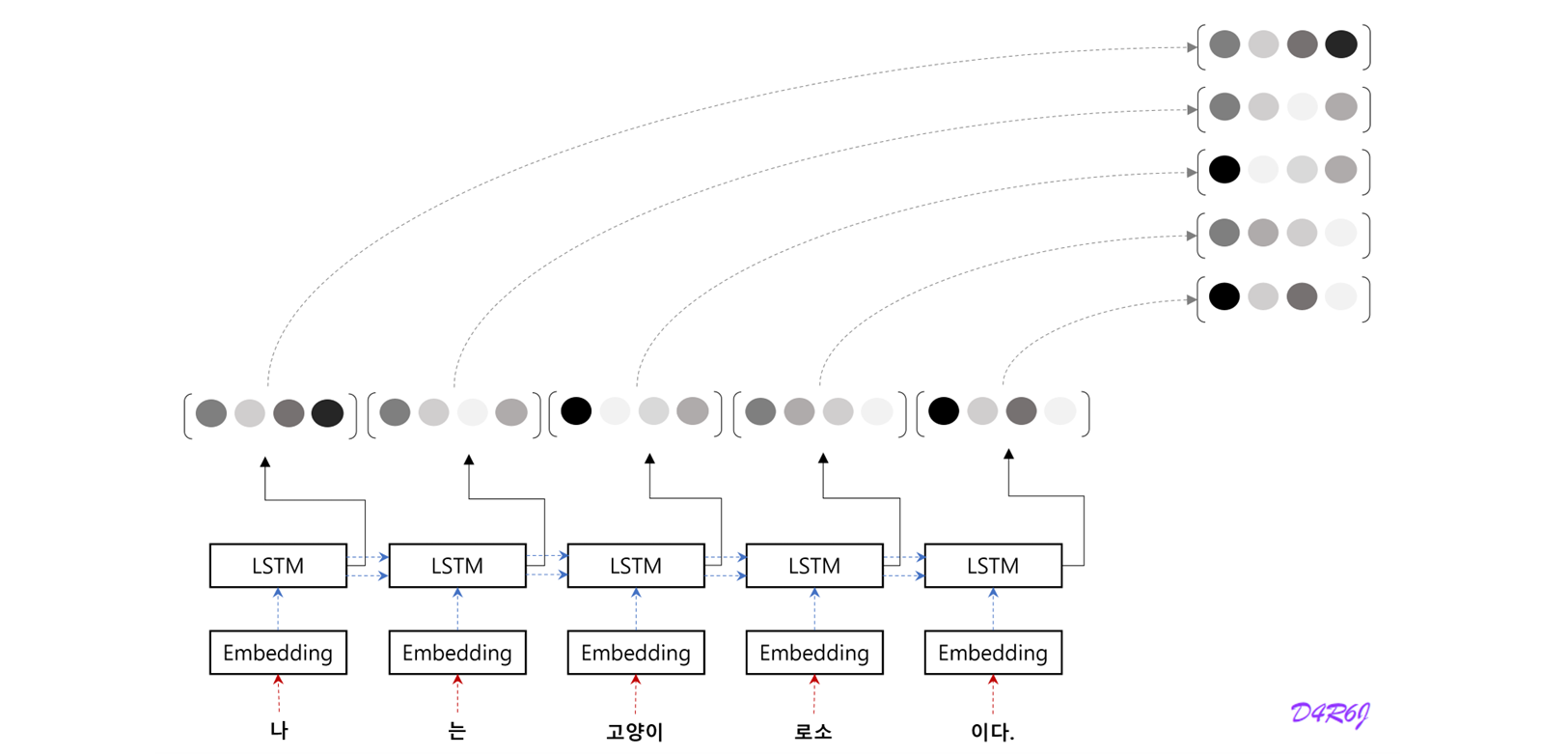
4. BiRNN (Bidirectional RNN)

long term dependency
"고양이" 에 대응하는 벡터에 "나", "는", "고양이" 까지 총 세단어의 정보가 encoding.
RNN 구조 특성상, 현재 time step 과 멀어지면 멀어질 수록, 해당 정보에 대한 손실이 커진다는 문제점.

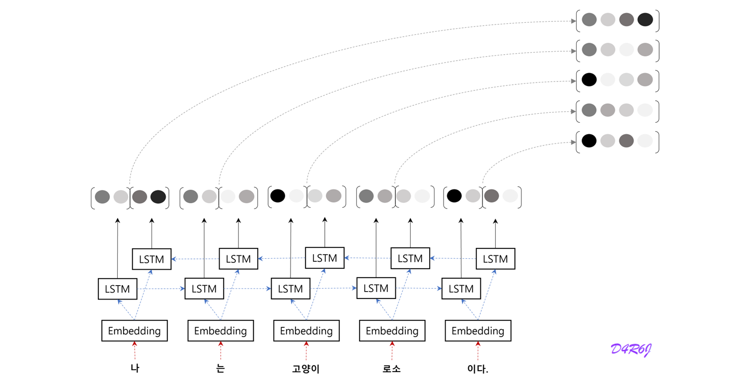
전체적인 균형을 생각하면, "고양이" 단어의 '주변' 정보를 균형 있게 담고 싶을 것.
양방향으로 처리, 각 단어에 대응하는 Hidden State Vector 에는 좌, 우 양쪽의 균형잡힌 정보를 encoding.

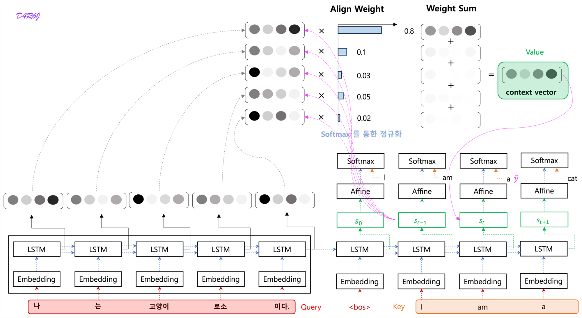
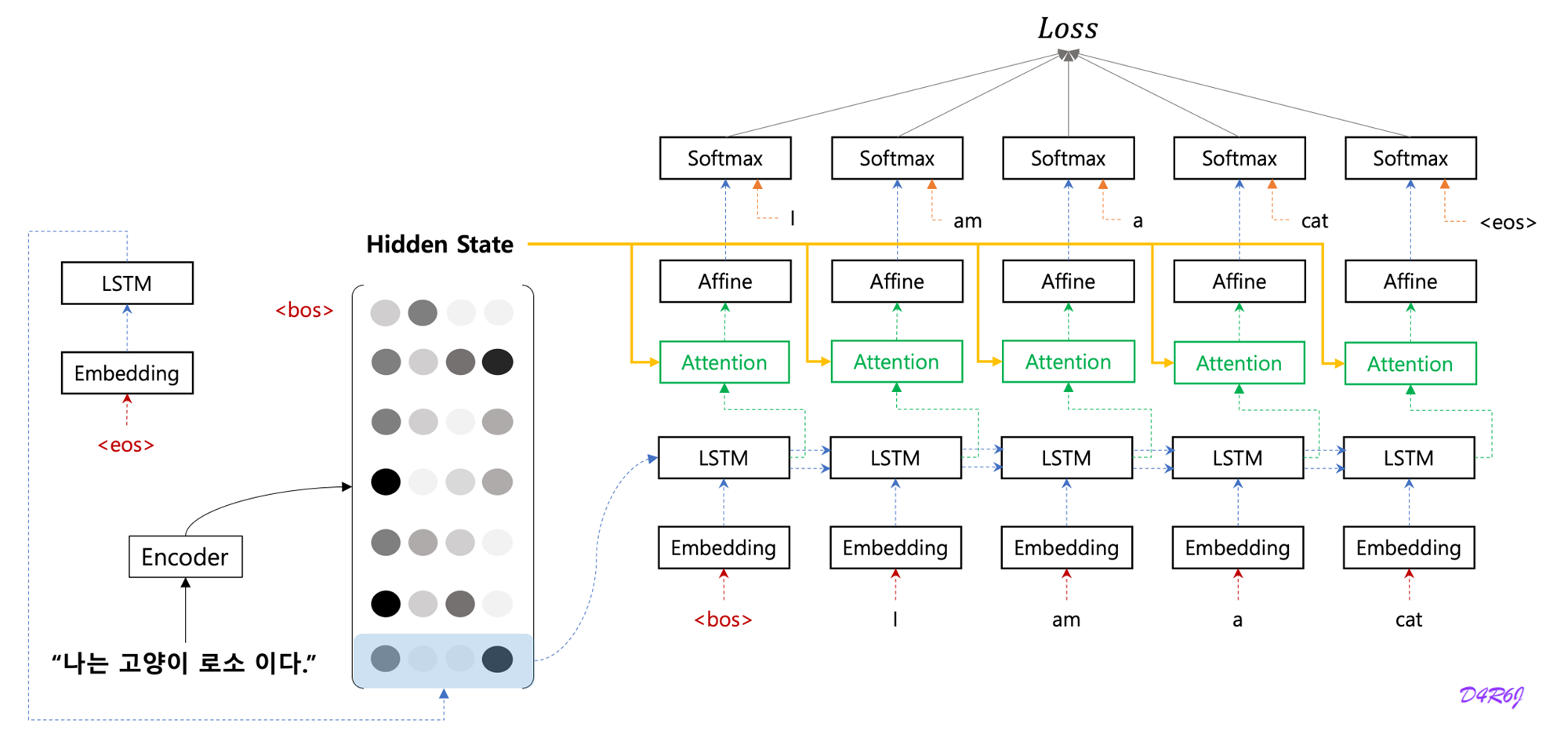
5. Attention

Encoder

LSTM 계층의 마지막 hidden state 만을 decoder 에 전달했다. 그러나 encoder 출력의 길이는 입력 문장의 길이에 따라 바꿔주는 게 좋다.

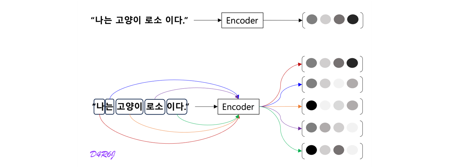
5 개의 단어가 입력 되었고, 이때 encoder 는 5개의 vector 를 출겨한다. '하나의 고정 길이 벡터' 제약에서 해방된다.
문장의 길이에 관계 없이 dyanmic 하게 정보를 encoding 이 가능하게 된다.

Decoder

source sentence 의 sequence of vector 를 이용하여 decoder 가 decoding 이 가능하게 된다.
decoding step 1.
- Encoder 의 LSTM (RNN) 계층의 마지막 hidden state 만을 이용한다. 마지막 줄만 빼내어 decoder 에 전달.

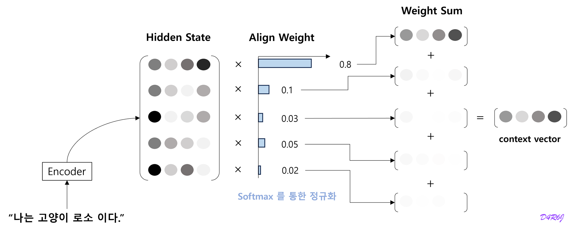
hidden state matrix 모두를 활용하도록 개선.
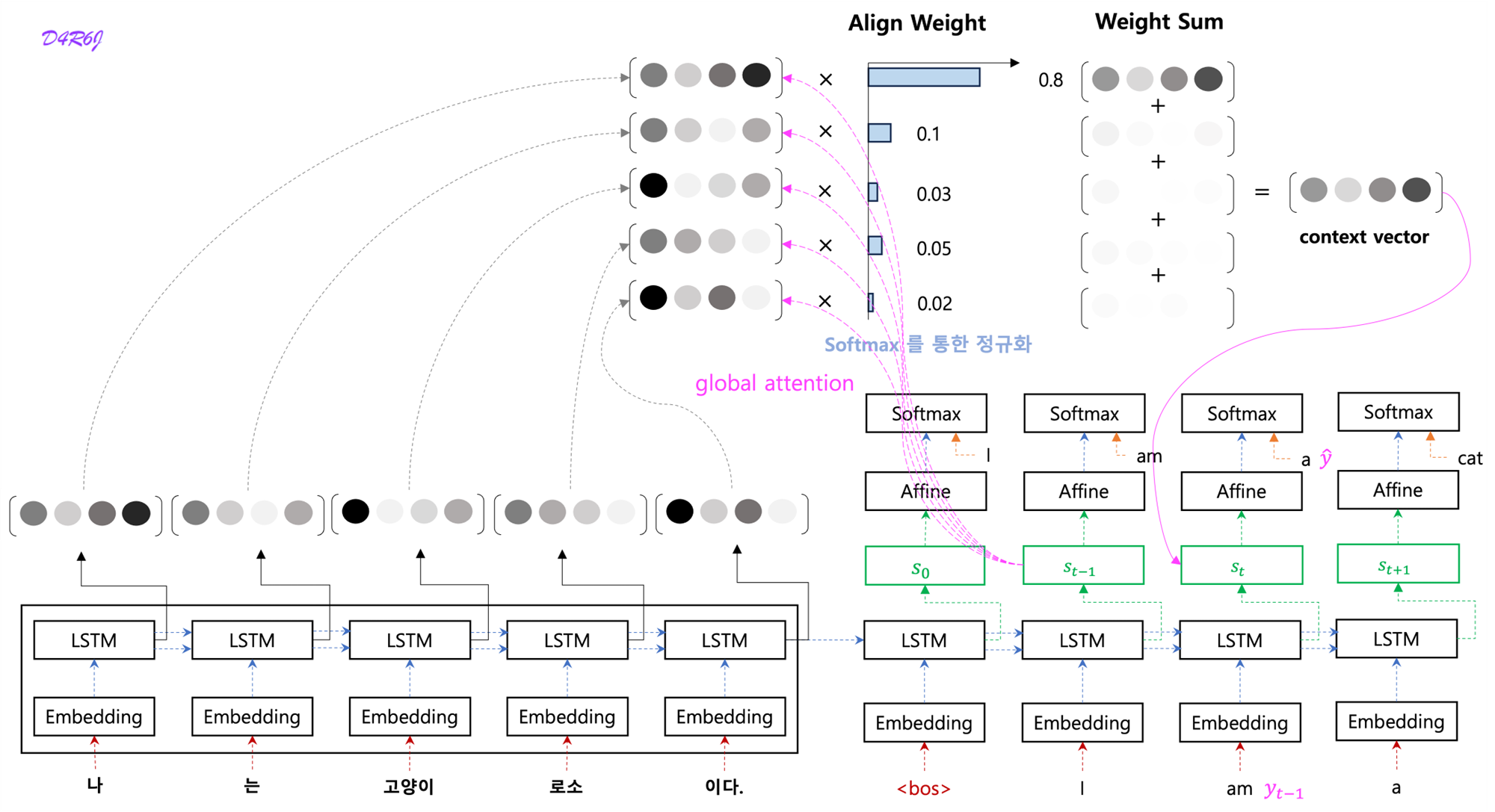
- 나 = I, 고양이 = cat 과 같이 입력과 출력의 여러 단어 중 어떤 단어끼리 서로 관련되어 있는가를 seq2seq 에게 학습 시킬 수 없을까?
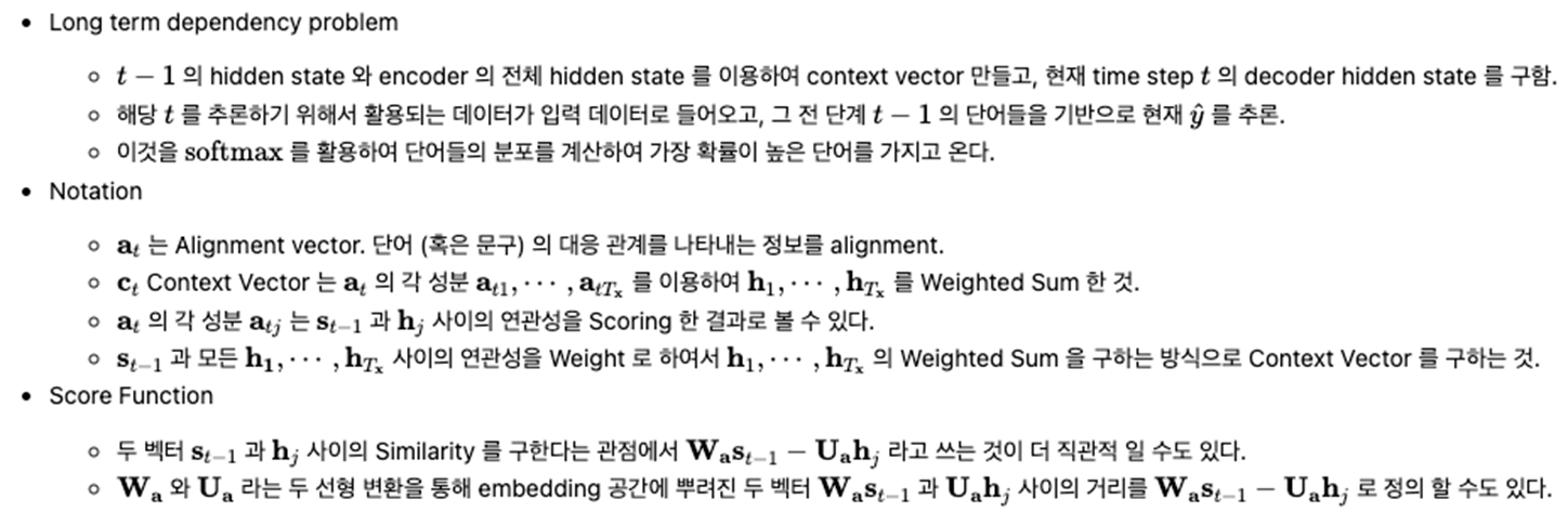
- 단어 (혹은 문구) 의 대응 관계를 나타내는 정보를 alignment.
- 목표는 '도착어 단어' 와 대응 관계에 있는 '출발어 단어' 의 정보를 골라내는것, 그리고 그 정보를 이용하여 번역을 수행하는 것.
- 정보를 골라내는, 선택하는 작업은 미분할 수가 없어서 모든 것을 선택하고 중요도를 나타내는 '가중치' 를 별도로 계산.

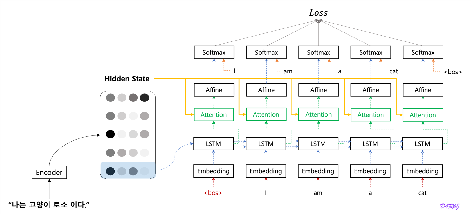
decoding step 2.
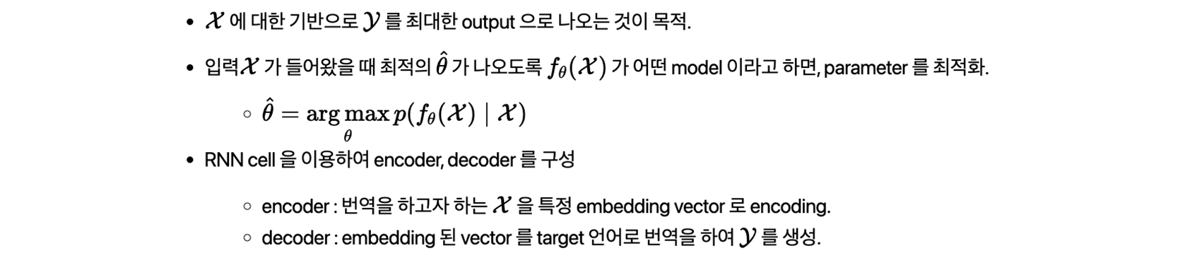
- Attention mechanism 을 이용하여 확률 모델 $\hat{\mathbf{y}}$ 를 기본 RNN 모델을 이용하여 모델링 하면 아래와 같다.

\hat{\mathbf{y}} = p(\mathbf{y}_t|\mathbf{y}_0, \cdots, \mathbf{y}_{t-1}, \mathcal{X}) = {\rm Softmax(\mathbf{W}_y\mathbf{s}_t + \mathbf{b}_y)}

\mathbf{s}_t = {\rm tanh(\mathbf{W}_{ys}\mathbf{y}_{t-1} + \mathbf{W}_{ss}\mathbf{s}_{t-1} + \mathbf{W}_{cs}\mathbf{c}_{t} + \mathbf{b}_s)}

{\rm where \; \mathbf{y}_0 = <sos>Token, \;\mathbf{s}_0 = \mathbf{0}, \; \mathbf{c}_t={\rm Attn(\mathbf{s}_{t-1}, \mathbf{H}), \; \mathbf{H}=[\mathbf{h}_1;\cdots;\mathbf{h}_{T_x}}]\in\mathbb{R}^{d \times T_x}}

Notation
- $d$ 는 encoder RNN Hidden State Vector 의 dimension.
- $\mathbf{y}_0$ 는 문장 embedding 을 사용하지 않고 문장의 시작점을 나타내는 새로운 token 을 사용.
- $\mathbf{s}_0$ 는 평범한 RNN 처럼 Zero Vector 를 사용하게 된다.
- $\mathbf{c}_t$ 는 어떤 계산이 되며, Attention 을 이용하게 된다.
- 필요한 정보에만 주목하여 그 정보로부터 시계열 변환을 수행하는 것이 목표. 이 구조를 attention.

6. Bahdanau

\mathbf{c}_t = \sum^{T_{\rm x}}_{j=1}\mathbf{a}_{tj}\mathbf{h}_{j} = \mathbf{Ha}_t

\mathbf{a}_t = {\rm Softmax \left( \left( Score(\mathbf{s}_{t-1}, \mathbf{h}_j\right)^{T_{\rm x}}_{j=1}\right)} \in \mathbb{R}^{T_{\rm x}}

{\rm Score}(\mathbf{s}_{t-1}, \mathbf{h}_j) = \mathbf{v}^{\top}{\rm tanh}(\mathbf{W}_a\mathbf{s}_{t-1} + \mathbf{U}_{\mathbf{a}}\mathbf{h}_j)

Result

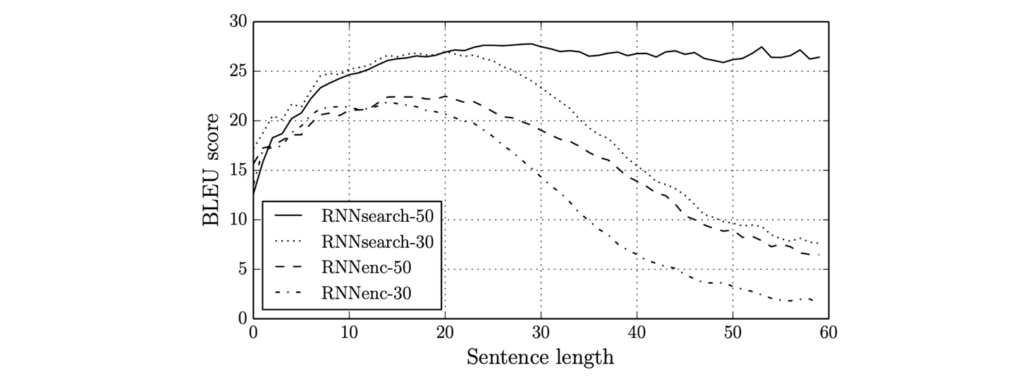
RNNsearch : attention mechanism 이 추가된 model.
RNNenc : attention mechanism 이 없는 model.
50, 30 : 학습 데이터의 길이
attention mechanism 과 문장의 길이가 긴 데이터로 학습한 모델이 성능이 제일 좋다.

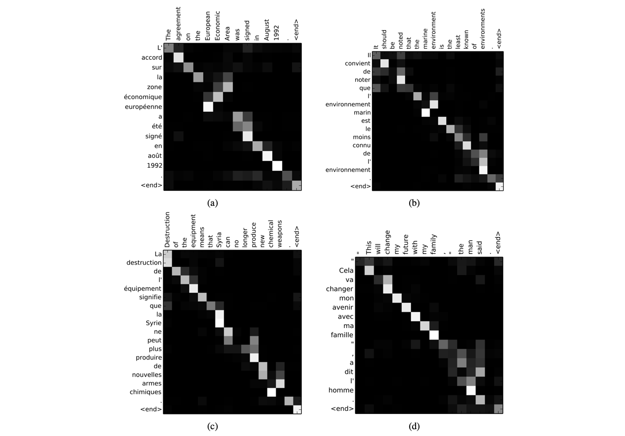
SVO (Subject Verb Object) 구조로 되어있는 english, french 두 개의 언어를 번역, diagonal term 이 highlighting. 좀 다른 영역도 있지만, 그 근방에서 보여진다.
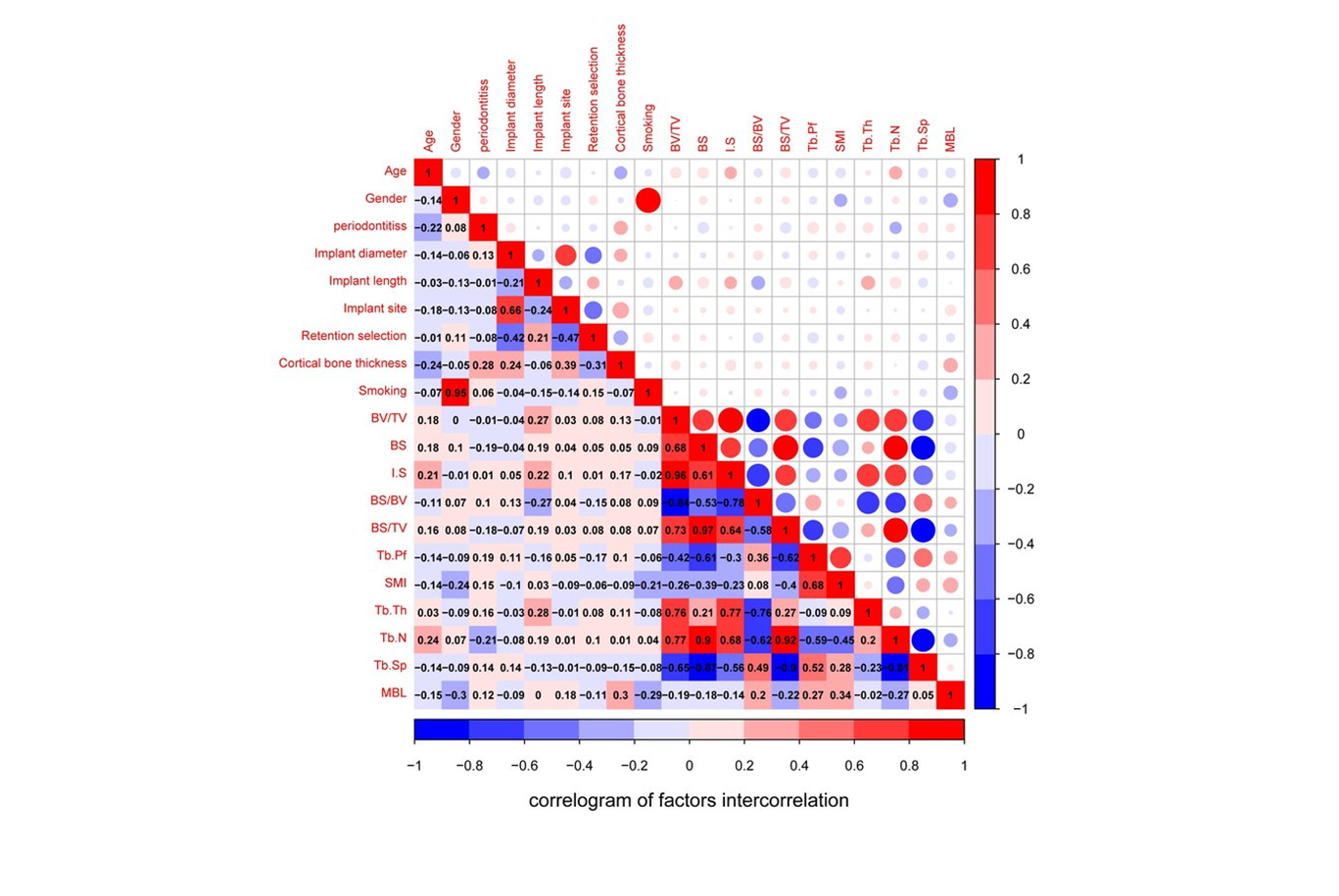
attention map 은 correlogram 과 비슷하다.

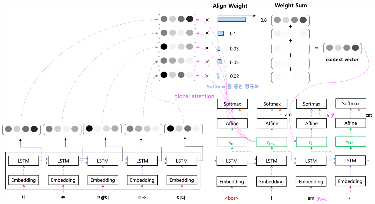
7. Luong

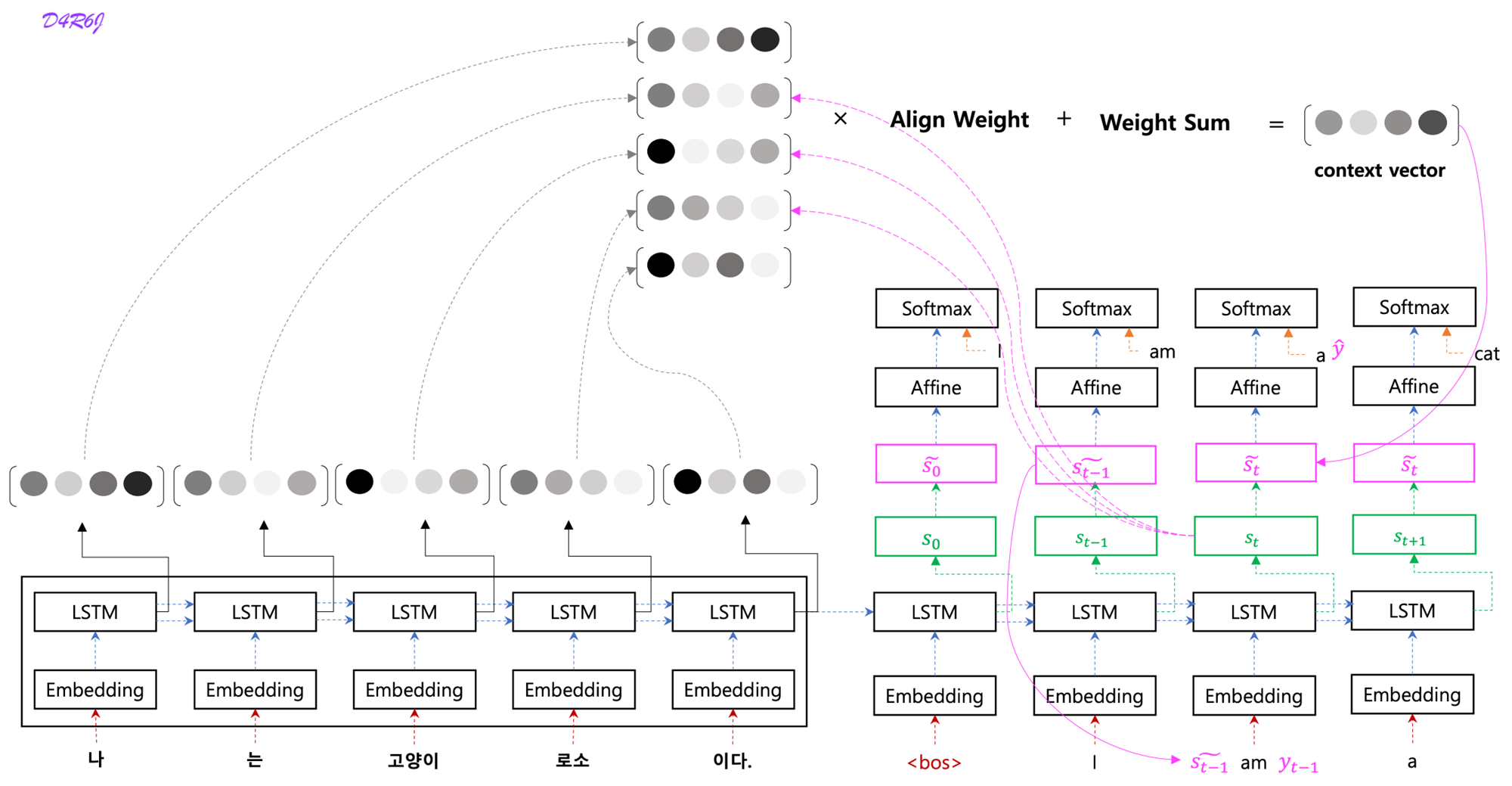
context vector 를 구할 때, $t$ 시점의 hidden state 를 활용하여 만듬.
output 을 예측할 때, 현재 시점의 hidden state 를 활용하는 것이 아니라 중간 단계인 $\tilde{s}$ 를 활용하여 output 을 예측.
input feeding 은 input 시에 $t-1$ 시점의 $\tilde{s}_{t-1}$ 를 같이 활용.
bahdanau 에서는 $\mathbf{c}_t$ 시점의 decoder hidden state 가 입력 값으로 들어가기 때문에 다음 step 으로 넘어가기 위해서 context vector 가 다 만들어질 때 까지 대기.
luong 에서는 이 문제를 두개의 hidden state 로 분리해서 재귀적으로 다음 step 으로 넘어가는 것이 수월해졌고, context vector 연산을 기다리지 않도록 효율적으로 바뀜.

\mathbf{c}_t = \sum^{T_{\rm x}}_{j=1}\mathbf{a}_{tj}\mathbf{h}_{j} = \mathbf{Ha}_t

\mathbf{a}_t = {\rm Softmax (\mathbf{W}_{y}\tilde{\mathbf{s}}_t + \mathbf{b}_y)}

\tilde{\mathbf{s}}_t = {\rm tanh}(\mathbf{W}_\mathbf{ss}\mathbf{s}_{t} + \mathbf{W}_\mathbf{cs}\mathbf{c}_t + \mathbf{b}_s)

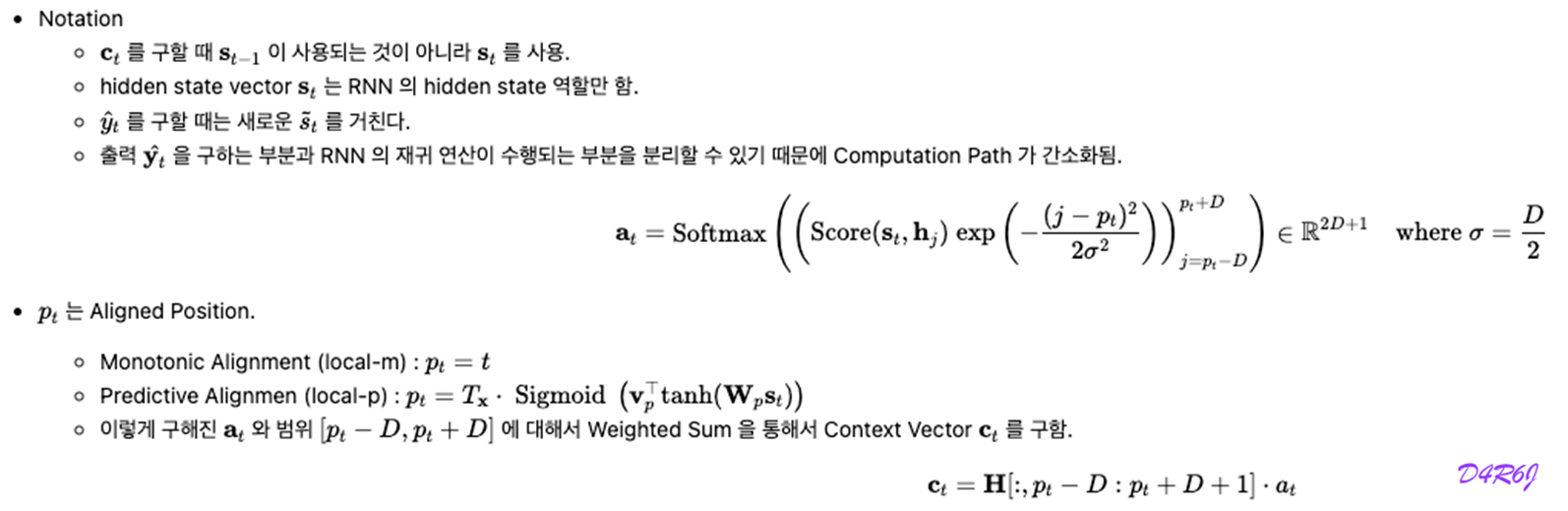
Monotonic Alignment : $n$ 번째의 input 에 대해 몇 번째의 Output 을 주목해야 하는지 계산 하는 방식.
Predictive Alignment : Decoder 의 Hidden state 를 sigmoid 함수를 이용하여 몇 번째 output 을 주목해야 하는지 계산하는 방식.
- $p_t$ Aligned position 의 최종 계산값이 2.5 가 나왔다면 Output Sequence 중 3 번째를 주목하는 방식. Filter 는 Gaussian 적용.

Result

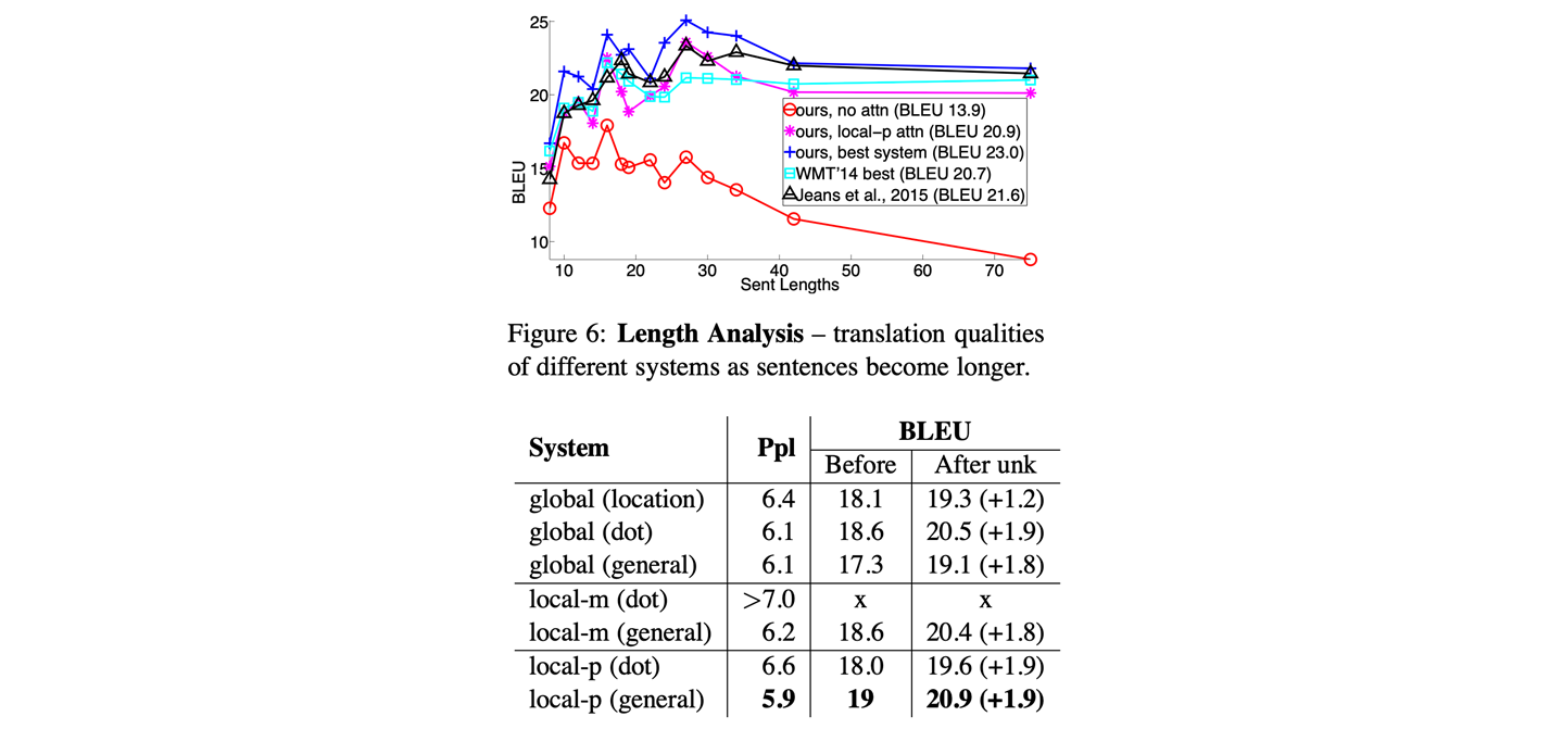
문장의 길이 별 BLEU score 가 어떻게 되는지,
- 맨 아래 graph 는 attention 이 없어서 문장이 길어질 수록 성능에 대한 손실이 커진다.
- attention 이 들어갔을 때, 문장의 길이에 상관 없이 성능을 어느 정도 유지할 수 있다.
- long term dependence problem 을 어느 정도 완화했다.
ppl : perplexity ( 수치가 낮을 수록 ), bleu ( 수치가 높을 수록 ) 좋다.
global attention 보다 local attention 이 효과적이다. $\rightarrow$ 부분적 으로만 봤을 때 좀 더 좋은 성능이 난다. (주장)
input fedding : 전 time step $\tilde{\mathbf{s}}_{t-1}$ 를 input 과 같이 concat 해서 입력 시 성능이 좀 더 좋다.
결과 해석에 대해서 attention map 을 활용하여 모델의 해석 가능성에 어느 정도 기여를 했다.

8. [B]ahadanau vs [L]uong

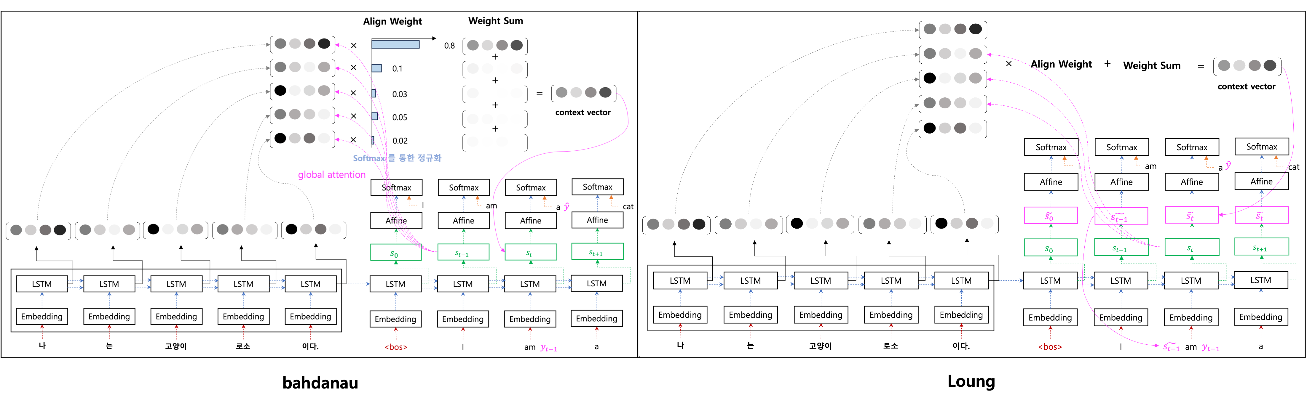
a. context vector 의 재료가 다르다.

[B] : 전 단계의 decoder hidden state 를 사용.
[L] : 현재 단계의 decoder hidden state 를 사용.

b. context vector 를 만드는 과정에서 연산하는 score 함수, encoder 와 decoder 의 유사도를 비교하는 함수 설정.

[B] : MLP 를 활용, encoder, decoder 의 hidden state 의 유사도 연산.
[L] : 3 가지 score 를 제시 :

{\rm score}(h_t, \bar{h}_s) \left \{ \begin{aligned} &h^{\top}\bar{h}_s \\ &h^{\top}W_a\bar{h}_s \\ &W_a[h_t;\bar{h}_s] \end{aligned} \right.

c. decoder 의 output 예측 시

[B] : decoder hidden state 자체를 활용.
[L] : 중간 단계의 $\tilde{s}_t$ 를 활용.

d. encoder hidden state 를 보는 범위가 다름.

[B] : encoder 전체 범위를 다 보는 모델, global attention.
[L] : decoder 현재 time step 의 주변에 있는 encoder 의 hidden state 만 보는 모델, local attention.

e. 정보의 흐름

[B] : 단방향으로 정보가 흐름.
- 전 단계 $t-1$ 의 hidden state 에서 현재 단계의 hidden state 로 넘어가기 위해 context vector 를 꼭 연산.
1. $s_{t-1}$ 에서
2. align weight ${a_t}$ 를 구하고,
3. context vector ${c_t}$ 를 만들어서,
4. 현재 decoder hidden state 의 입력 값으로 들어간다.
[L] : 수평, 수직으로 정보가 흐름.
- 재귀적으로 decoder hidden state 가 연산 하는 것은 두고, output 에서 context vector 를 활용할 때는 따로 $\tilde{s}$ 연산.
1. $s_{t-1}$ 에서
2. align weight ${a_t}$ 를 구하고,
3. context vector ${c_t}$ 를 만들어서,
4. context vector 가 output 을 예측할 때 $\tilde{s}$ 의 재료로 만들어지게 된다.
- 이와 같이 두개의 방향으로 나누어져 구분하면 context vector 전에 재귀적으로 decoder hidden state 가 진행할 수 있다.

f. Input feeding approch [L]

input 의 단어 vector 와 그 전 단계의 $\tilde{s}_{t-1}$ decoder hidden state 까지 concatenation 해서 입력으로 들어감.
그 전 단계에서 연산한 align weight, decoder state 와 encoder hidden state 간의 관계 정보도 넣어서 다양한 정보를 활용.

9. Conclusion

Main Contribution

Long term(range) dependency problem 완화.
해석 가능성
- Attention map 을 활용하여 이 모델의 결과가 어떻게 이렇게 되었는지 해석할 수 있게 되었다.
- 해석 가능성에 대한 어느정도를 기여하게 되었다.
Query, Key, Value