[ Transformer ] paper, code review

Attention Is All You Need (paper)

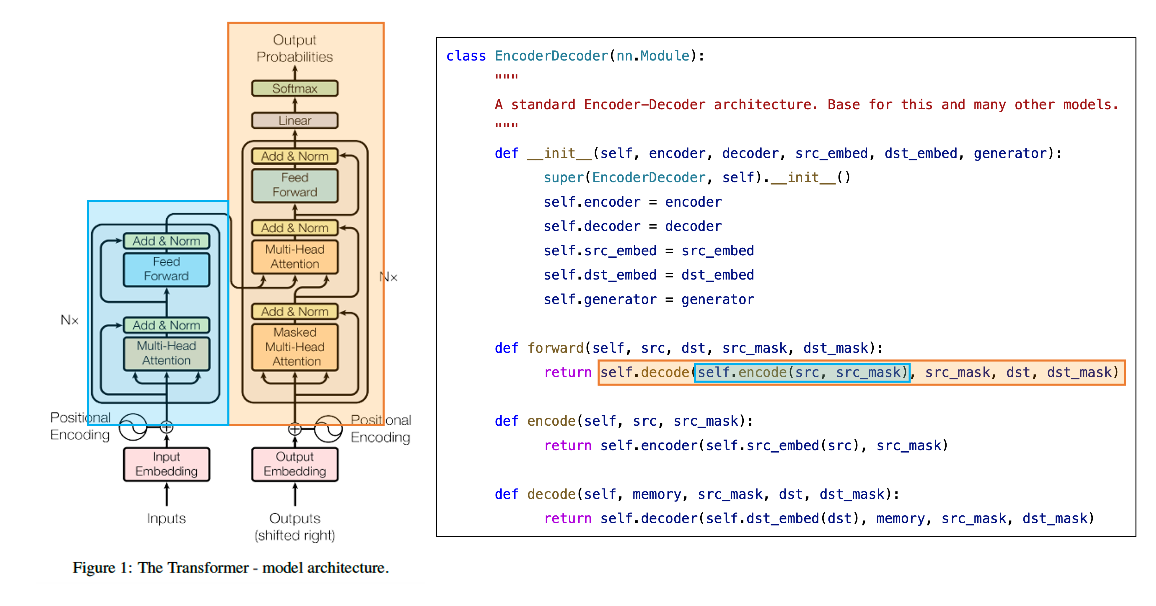
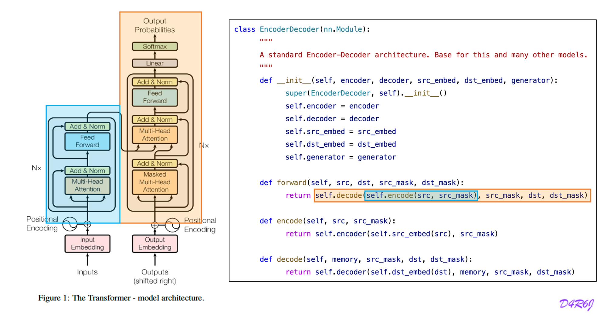
1. Model Architecture

• Input sequence of symbol representation $\rightarrow (x_1, \cdots, x_n)$
• sequence of continuous representations $\rightarrow \mathbf{z} = (z_1, \cdots, z_n)$
• Given $\mathbf{z}$, the decoder then generate an output sequence $\rightarrow (y_1, \cdots, y_m)$

---

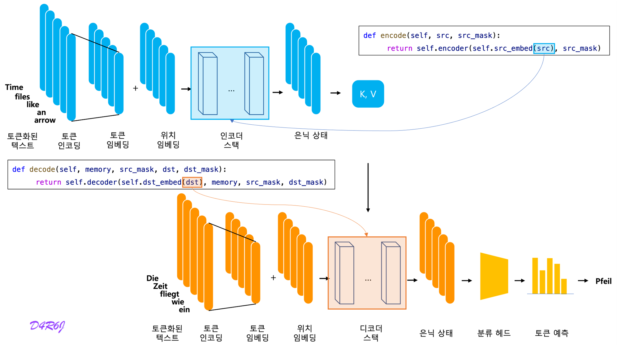
2. Encoder and Decoder Stacks

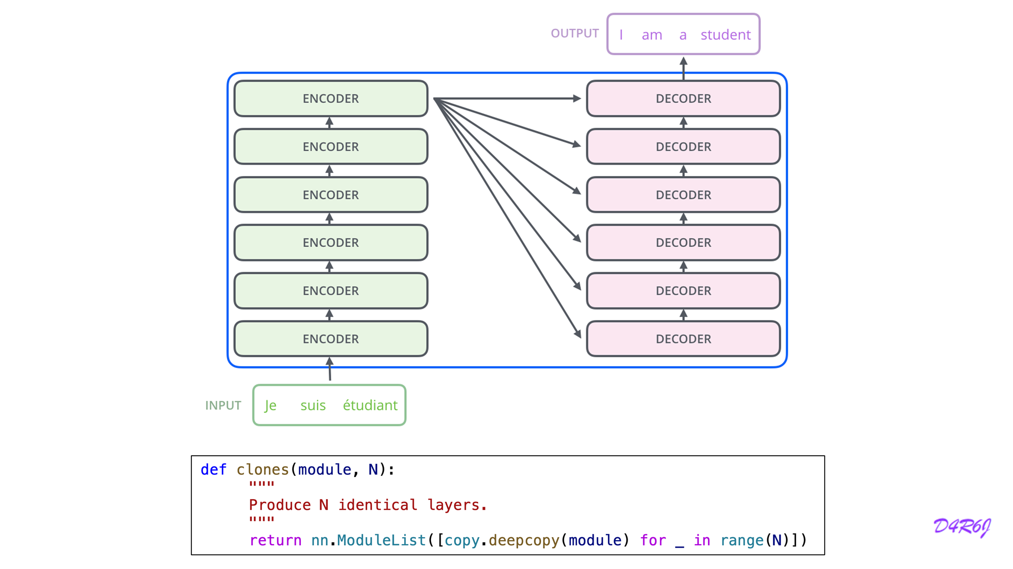
2-1. Encoder

• Encoder is composed of a stack of $N=6$ identical layers.

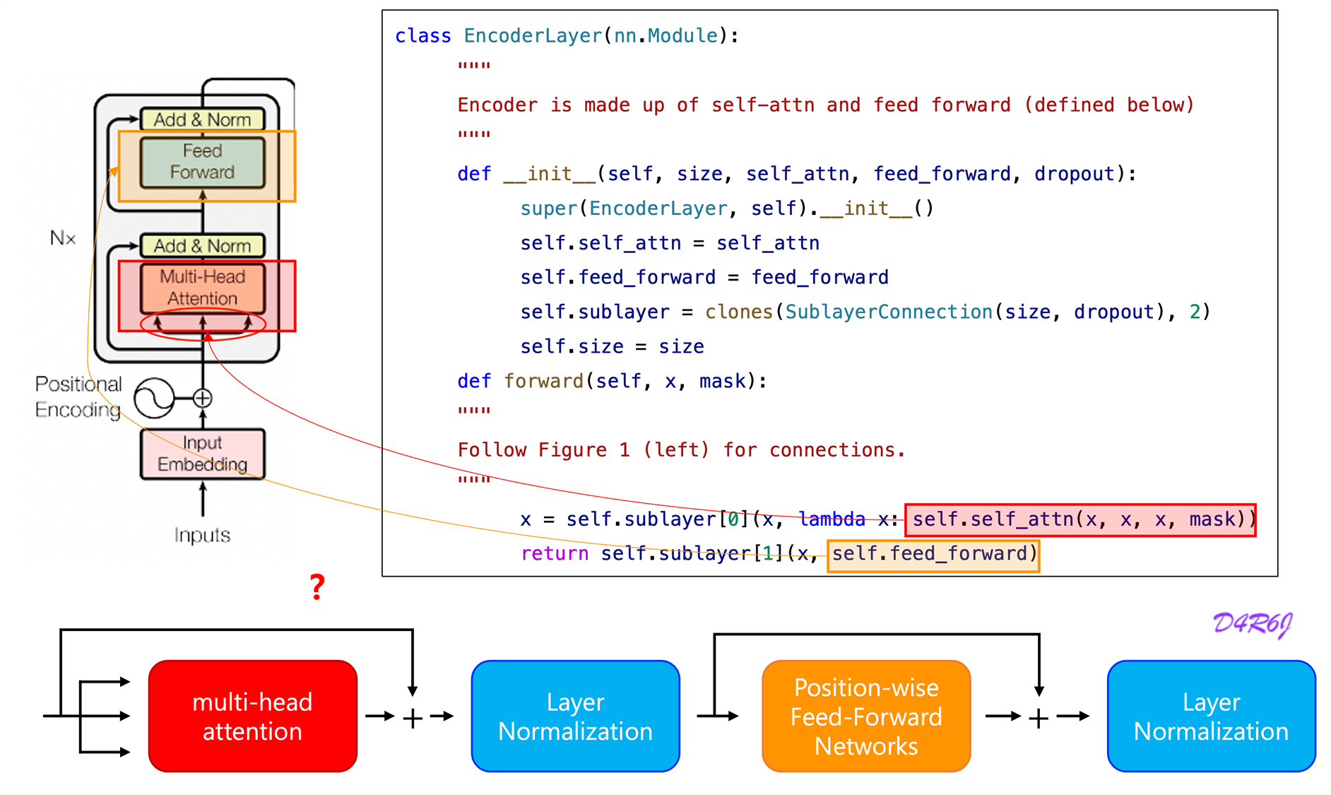
1. A multi-head self-attention mechanism.
2. simple, position-wise fully connected feed-forward network.

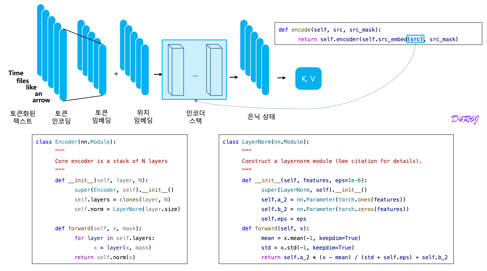
• Residual connection around each of the two sub-layers, followed by layer normalization.
• The output of each sub-layer is ${\rm LayerNorm}(x + {\rm Sublayer}(x))$

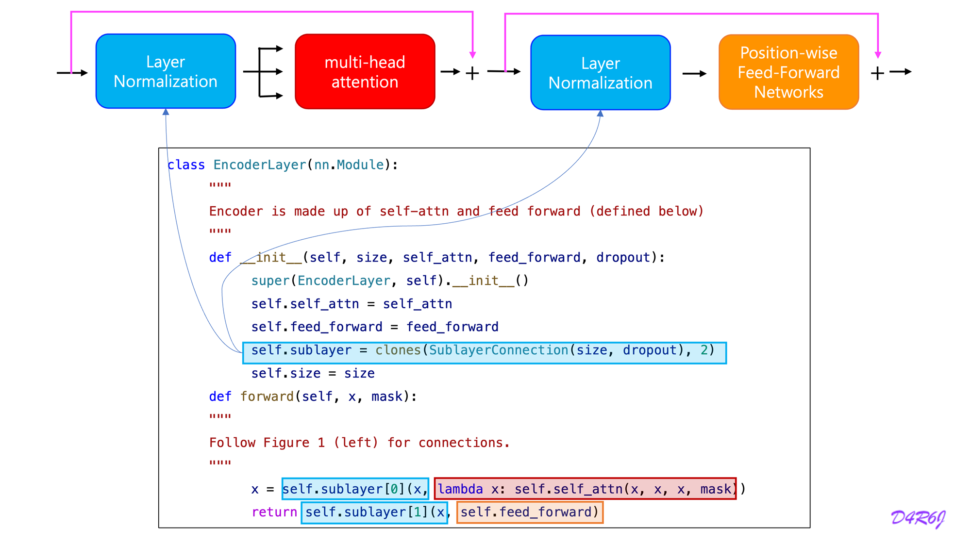
• To facilitate these residual connections, all sub-layers in the model, as well as the embedding layers, produce outputs of dimension $d_{model} = 512$

2-2. Decoder

• Decoder is also composed of a stack of $N=6$ identical layers.

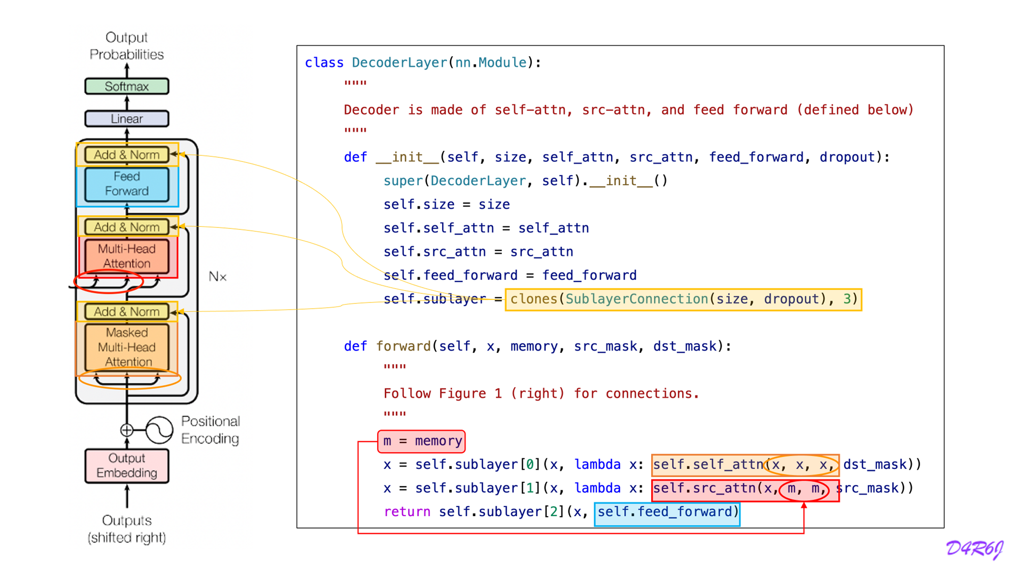
• The decoder inserts a third sub-layer, which performs multi-head attention over the output of the encoder stack.
• This masking, combined with fact that the output embeddings are offset by one position, ensures that the predictions for position $i$ can depend only on the known outputs at positions less than $i$.

---

3. Attention

• An attention function can be described as mapping a query and a set of key-value pairs to an output, where the query, keys, values, and output are all vectors.
• The output is computed as a weighted sum of the values, where the weight assigned to each value is computed by a compatibility function of the query with the corresponding key.

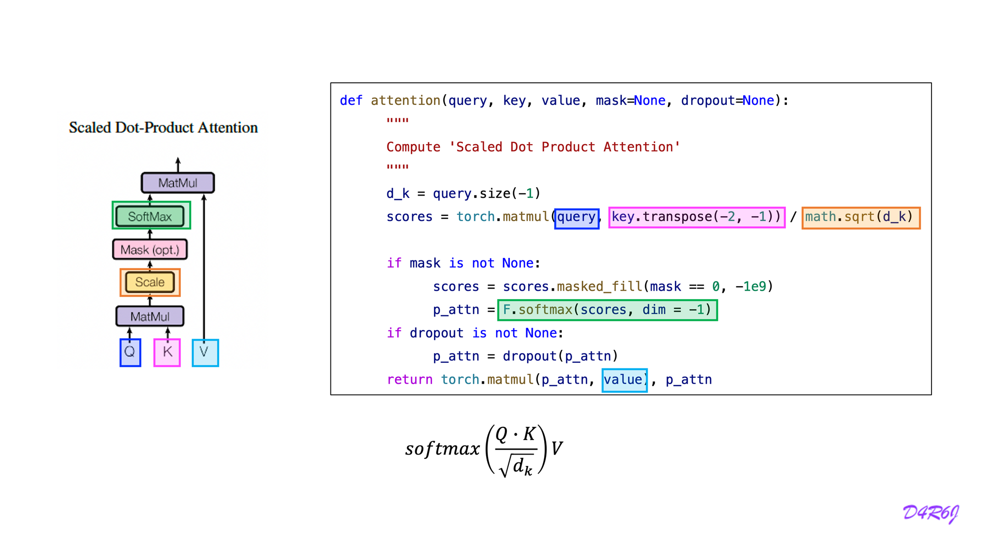
3-1. Scaled Dot-Product Attention

• The queries simultaneously, packed together into a matrix $Q$.
• The keys and values are also packed together into matrices $K$ and $V$.
  ${\rm Attention}(Q, K, V) = {\rm softmax}(\frac{QK^\top}{\sqrt{d_k}})V$

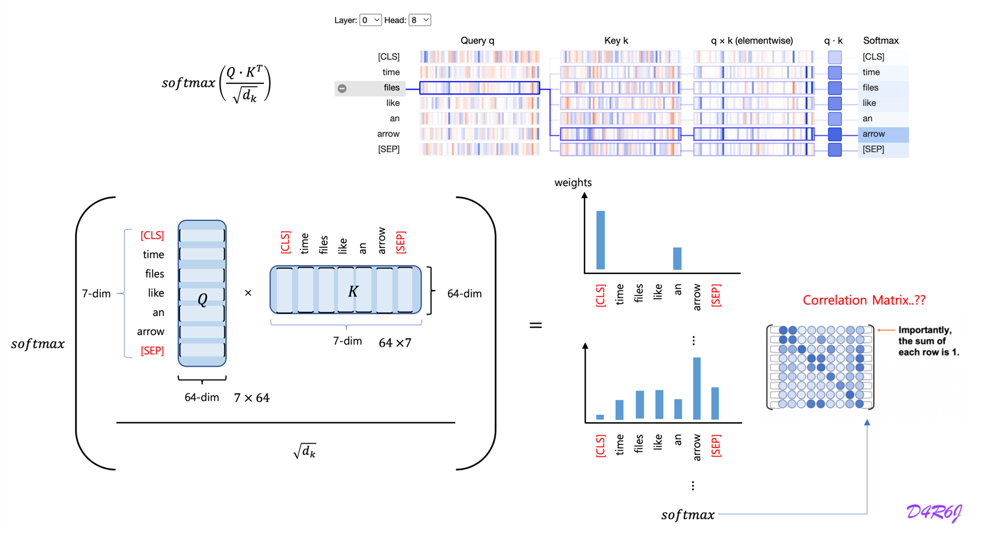
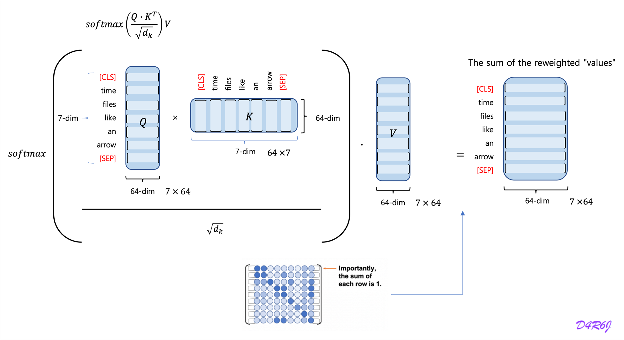
• Large values of $d_k$, the dot products grow large in magnitude, pushing the softmax function into regions where it has extremely small gradients.to counteract this effect, we scale the dot products by $\frac{1}{\sqrt{d_k}}$

• To illustrate why the dot products get large, assume that the components of $q$ and $k$ are independent random variables with mean $0$ and variance $1$. Then their dot product, $q \cdot k = \sum\limits_{i=1}^{d_k} q_ik_i$, has mean $0$ and variance $d_k$.

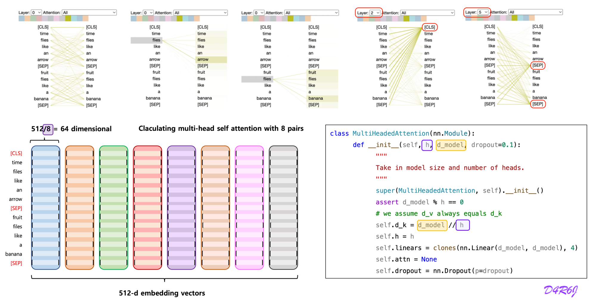
3-2. Multi-Head Attention

Multi-head attention allows the model to jointly attend to information from different representation subspace at different positions. with a single attention head, averaging inhibits this.

Where the projections are parameter matrices

and $W^{O} \in \mathbb{R}^{{hd_v}\times d_{model}}$

In this work we employ $h = 8$ parallel attention layers, or heads. For each of these we use $d_k = d_v = d_{model}/h = 64.$ Due to the reduced dimension of each head, the total computational cost is similar to that of single-head attention with full dimensionality.

---

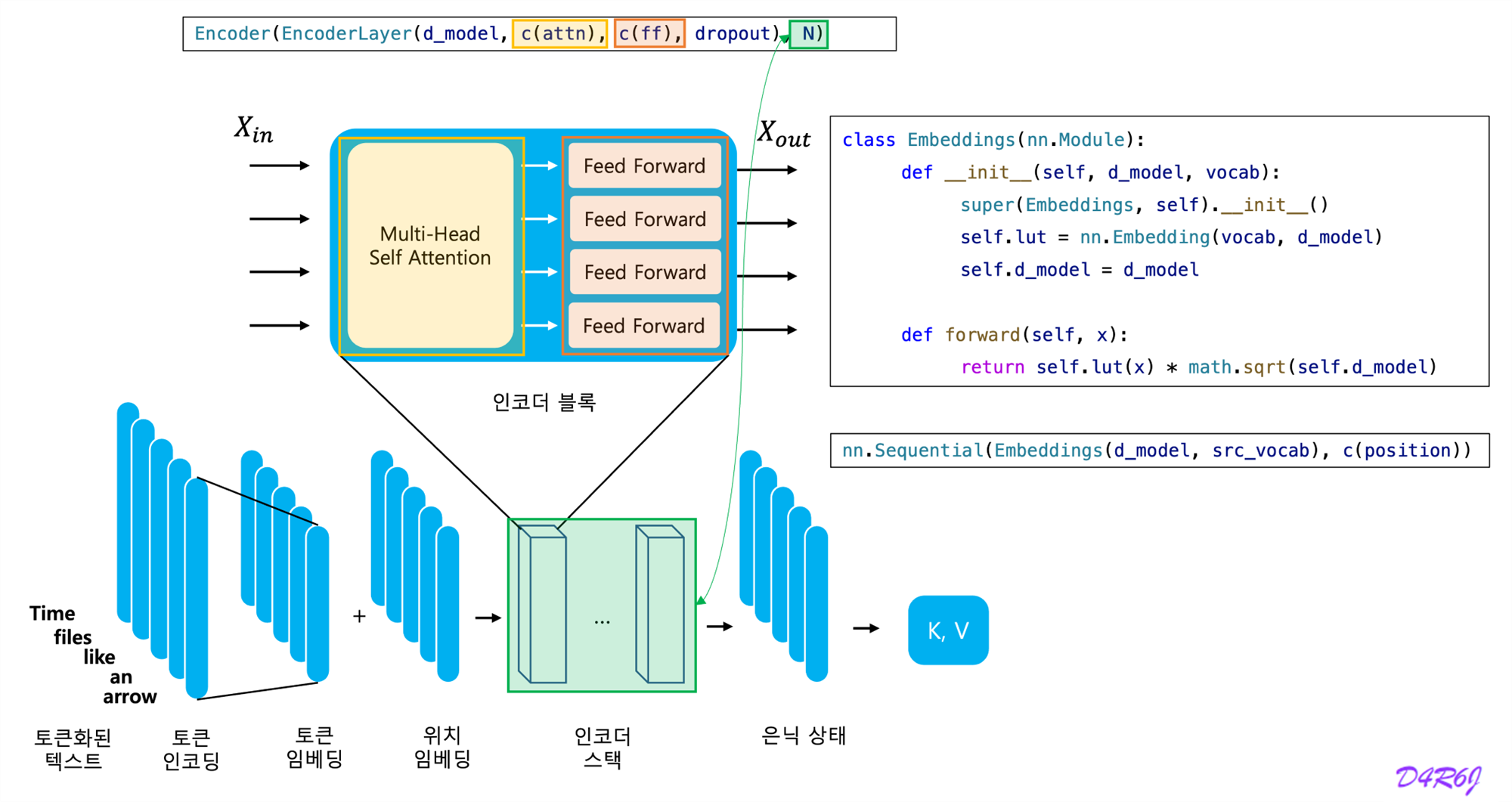
4. Position-wise Feed-Forward Networks

In addition to attention sub-layers, each of the layers in our encoder and decoder contains a fully connected feed-forward network, which is applied to each position separately and identically $(i.i.d ??)$ . This consists of two linear transformations with a ReLU activation in between.

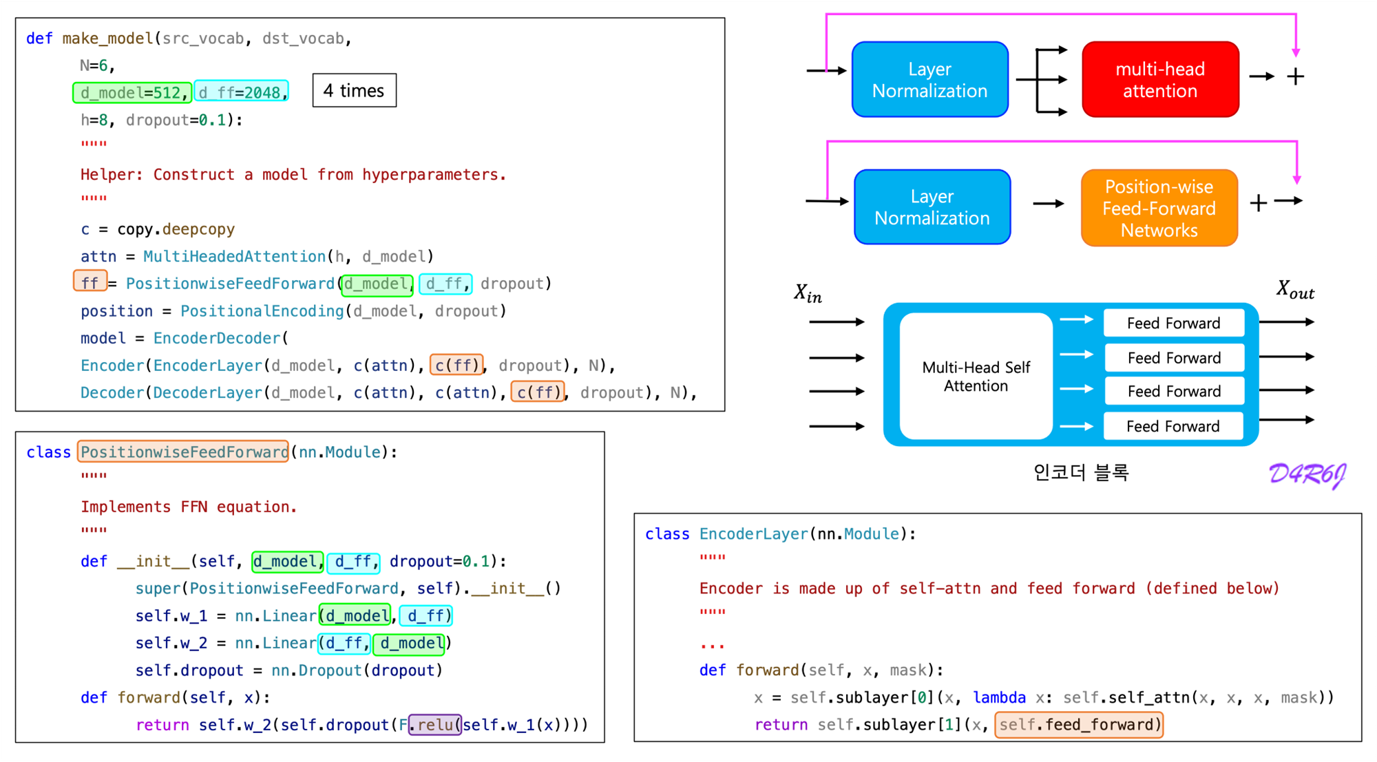
While the linear transformations are the same across different positions, they use different parameters from layer to layer. Another way of describing this is as two convolutions with kernel size $1$. The dimensionality of input and output is $d_{model} = 512,$ and the inner-layer has dimensionality $d_{ff} = 2048.$

---

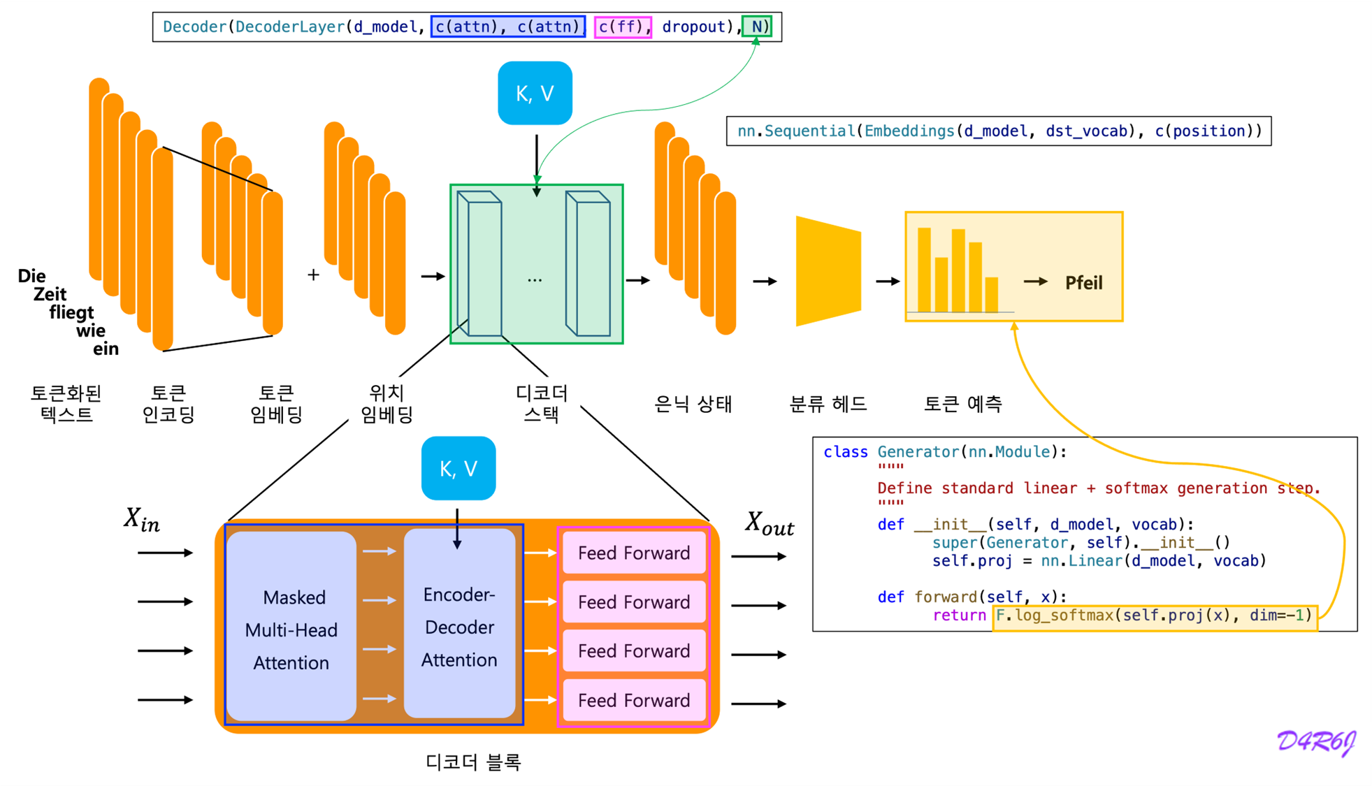
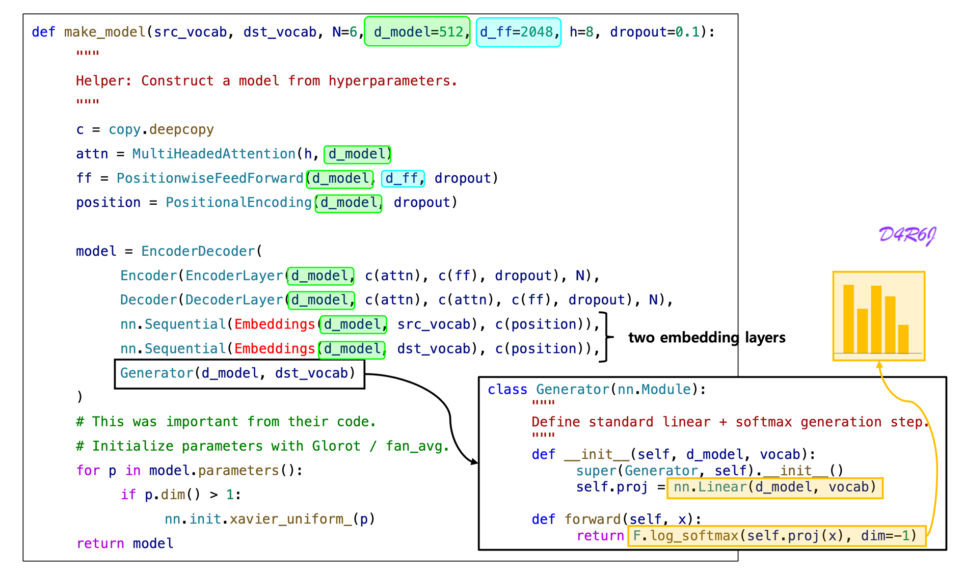
5. Embeddings and Softmax

• learned embeddings to convert tokens and output tokens to vectors of dimension $d_{model}.$

• The usual learned linear transformation and softmax function to convert the decoder output to predicted next-token probabilities.

• share the same weight matrix between the two embedding layers and the pre-softmax linear transformation, similar to..

---

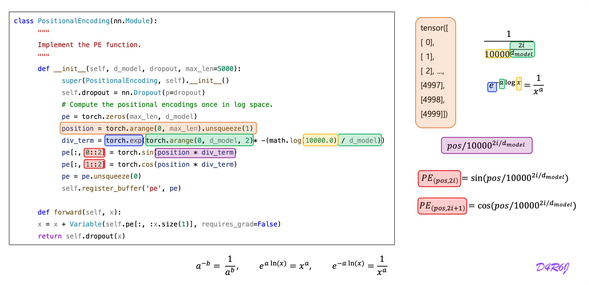
6. Positional Encoding

Since our model contains no recurrence and no convolution, in order for the model to make use of the order of the sequence, we must inject some information about the relative or absolute position of the tokens in the sequence.

In this work, we use sine and cosine functions of different frequencies:

We chose this function because we hypothesized it would allow the model to easily learn to attend by relative positions, since for any fixed offset $k, PE_{pos+k}$ can be represented as a linear function of $PE_{pos}.$

---

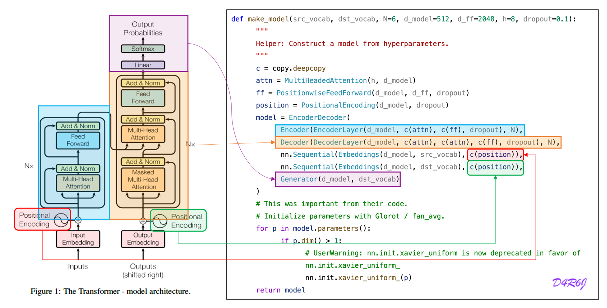
7. Full Model

Ref.

1. The Annotated Transformer (code)

2. Multi-head attention mechanism (blog)

3. The Illustrated Transformer (blog)

4. Natural Language Processing with Transformers (book)