실제 DeepSeek 구조에서 4 가지만 집고 넘어가보자.

1. MLA (Multi-Head Latent Attention)
   2. MoE (Mixture-of-Experts)
2. Knowledge Distillation
3. GRPO (Group Relative Policy Optimization)

Training Strong Models at Economical Costs

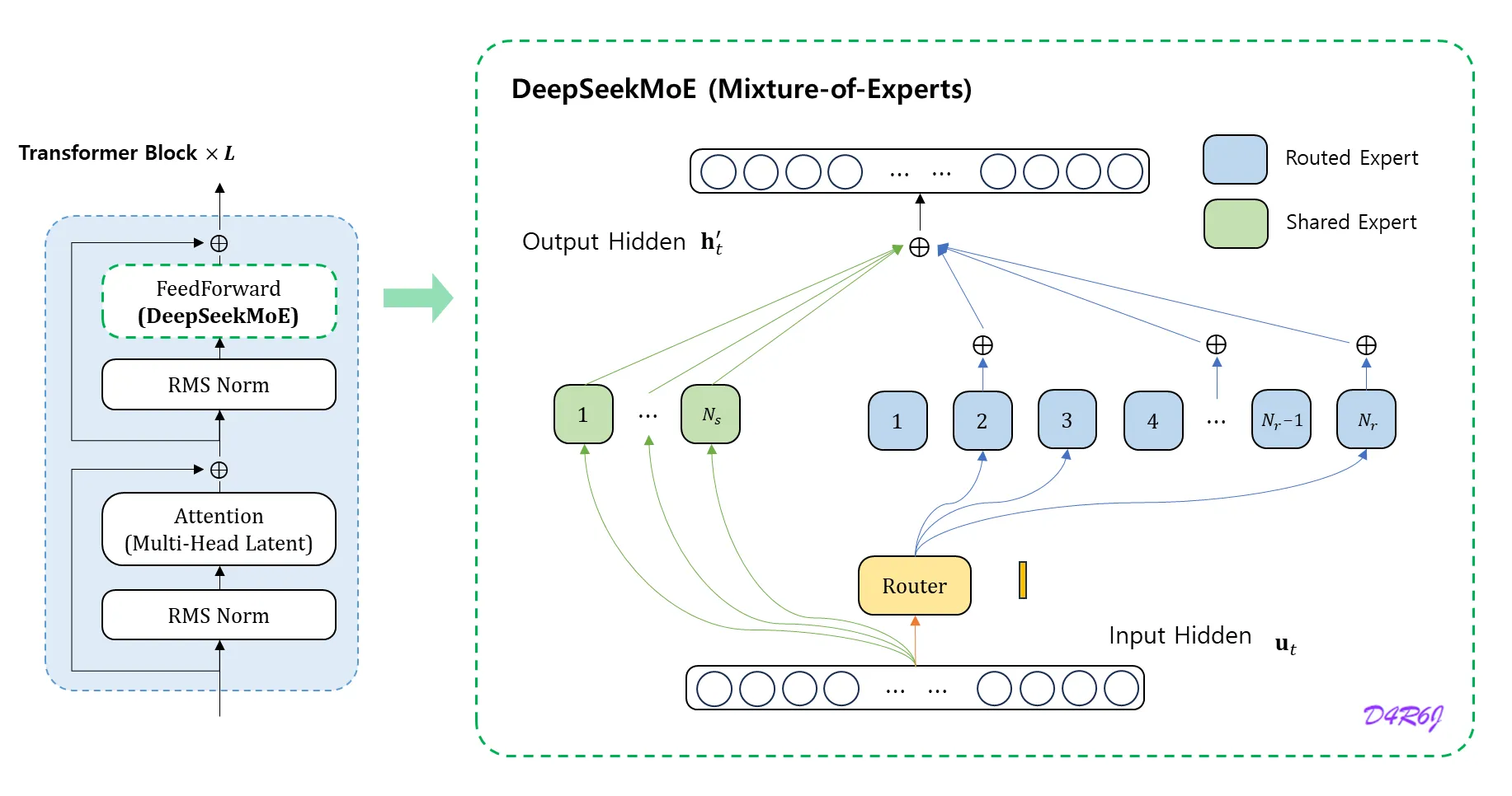
Basic Architecture

DeepSeekMoE 에는 두 가지 key idea 가 있다.

1. 전문가들을 더욱 세밀하게 세분화 하여 전문성을 더 높이고, 더 정확한 지식 습득을 하게 한다.

   → 세분화된 전문가.

2. 라우팅된 전문가들의 지식 중복성을 완화하기 위해서 일부 공유된 전문가 (shared) 를 격리한다.

   → 일부 전문가를 공유 전문가로 격리.

여기서 전문가 block 이 진짜.. 이게 다란 말인가..

• shared expert

  class MLP(nn.Module):
      """
      w1 (nn.Module): Linear layer for input-to-hidden transformation.
      w2 (nn.Module): Linear layer for hidden-to-output transformation.
      w3 (nn.Module): Additional linear layer for feature transformation.
      """
      def __init__(self, dim: int, inter_dim: int):
          super().__init__()
          self.w1 = ColumnParallelLinear(dim, inter_dim)
          self.w2 = RowParallelLinear(inter_dim, dim)
          self.w3 = ColumnParallelLinear(dim, inter_dim)
  
      def forward(self, x: torch.Tensor) -> torch.Tensor:
          return self.w2(F.silu(self.w1(x)) * self.w3(x))

• routed expert

  class Expert(nn.Module):
      """
       w1 (nn.Module): Linear layer for input-to-hidden transformation.
       w2 (nn.Module): Linear layer for hidden-to-output transformation.
       w3 (nn.Module): Additional linear layer for feature transformation.
      """
      def __init__(self, dim: int, inter_dim: int):
          super().__init__()
          self.w1 = Linear(dim, inter_dim)
          self.w2 = Linear(inter_dim, dim)
          self.w3 = Linear(dim, inter_dim)
  
      def forward(self, x: torch.Tensor) -> torch.Tensor:
          return self.w2(F.silu(self.w1(x)) * self.w3(x))

• 동일한 수의 활성화된 전문가 (activated) 와 전체 전문가 (total) parameter 를 사용 할 경우, DeepSeekMoE 는 GShard 와 같은 기존의 MoE 구조 보다 훨씬 더 뛰어난 성능을 발휘할 수 있다.

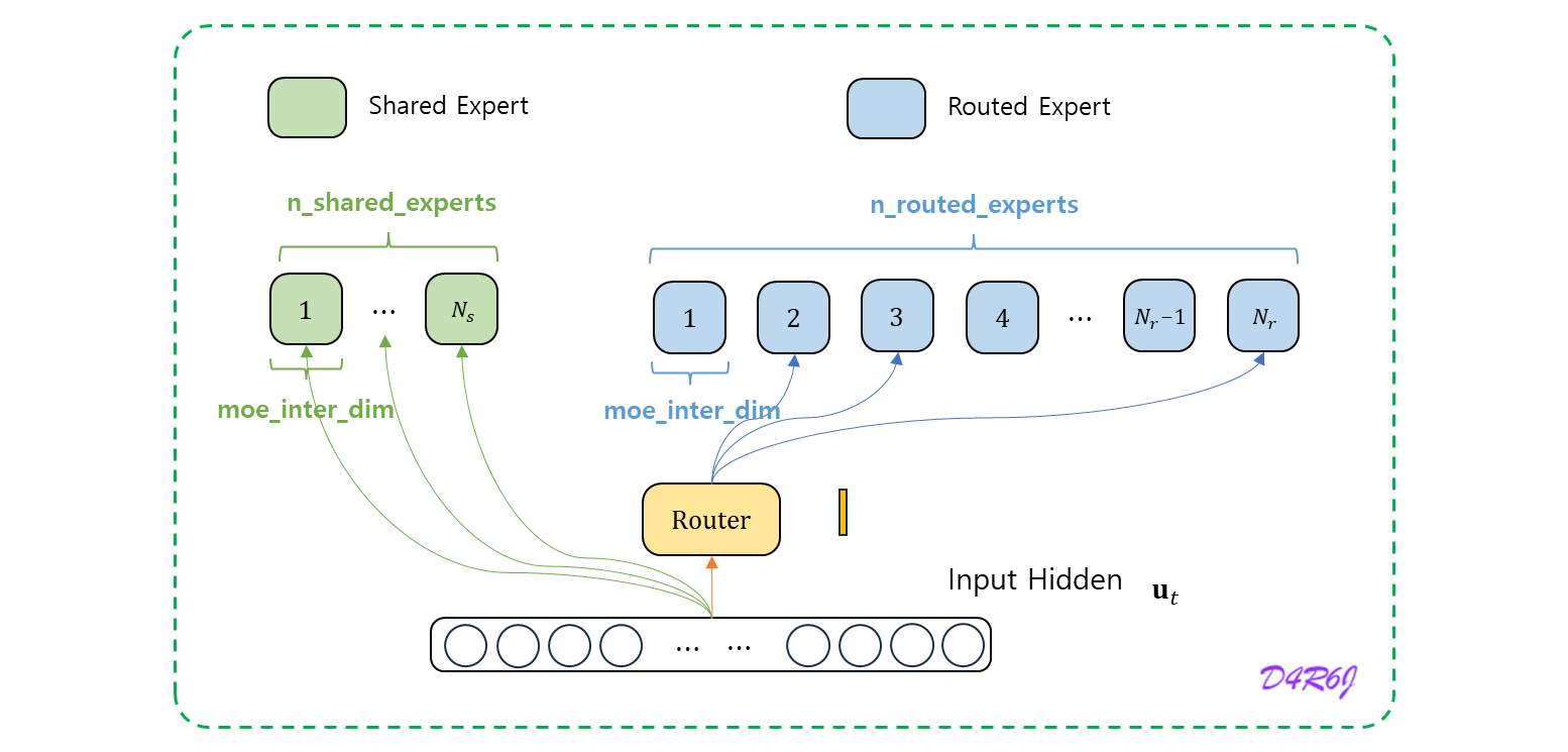
self.shared_experts = MLP(args.dim, args.n_shared_experts * args.moe_inter_dim)
self.experts = nn.ModuleList(
                   [
                       Expert(args.dim, args.moe_inter_dim) 
                           if self.experts_start_idx <= i < self.experts_end_idx 
                           else None 
                           for i in range(self.n_routed_experts)
                   ]
               )
y = torch.zeros_like(x)
z = self.shared_experts(x)

for i in range(self.experts_start_idx, self.experts_end_idx):
    if counts[i] == 0:
        continue
    expert = self.experts[i]
    idx, top = torch.where(indices == i)
    y[idx] += expert(x[idx]) * weights[idx, top, None]

• $\mathbf{u}_t$ 는 $t$ 번째 토큰의 FFN 입력
• $\mathbf{h}'$ FFN 출력

아래와 같이 계산한다.

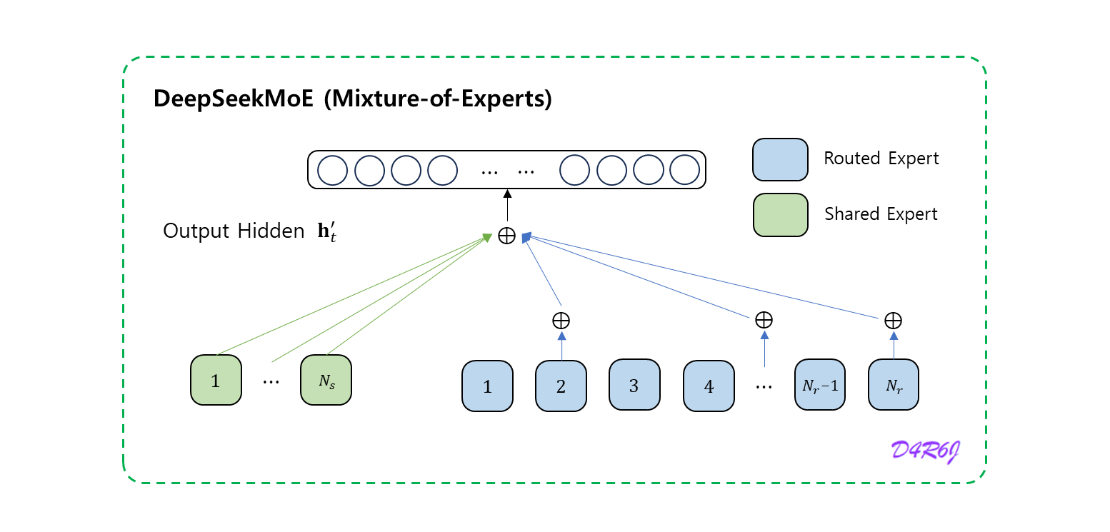
return (y + z).view(shape)

if self.score_func == "sigmoid":
    weights /= weights.sum(dim=-1, keepdim=True)

• 여기서 중요한 포인트는, softmax 일 때는 전체 합이 1 이 되지만, sigmoid 일 경우 값이 0 ~ 1 사이일 뿐, 그 합은 1이 아닐 수 있어서, 정규화 과정이 필요하다.

if self.bias is None:
    group_scores = scores.amax(dim=-1)
else:
    group_scores = scores.topk(2, dim=-1)[0].sum(dim=-1)
    
indices = group_scores.topk(self.topk_groups, dim=-1)[1]
# indices 아니면 모두 0 으로..
mask = torch.zeros_like(scores[..., 0]).scatter_(1, indices, True)
scores = (scores * mask.unsqueeze(-1)).flatten(1)

        scores = linear(x, self.weight)
        if self.score_func == "softmax":
            scores = scores.softmax(dim=-1, dtype=torch.float32)
        else:
            scores = scores.sigmoid()

• $N_s$ 는 공유된 전문가 (shared expert) 의 수

• $N_r$ 은 라우팅된 전문가 (routed expert) 의 수

• ${\rm FFN}_{i}^{(s)}(\cdot)$ 는 $i$ 번째 공유된 전문가

• ${\rm FFN}_{i}^{(r)}(\cdot)$ 는 $i$ 번째 라우팅된 전문가

• $K_r$ 은 활성화된 전문가 (activated export) 의 수

• $g_{i,t}$ 는 $i$ 번째 전문가의 게이트 값 (gate value)

• $s_{i, t}$ 는 token 전문가의 친밀도 (affinity)

• $\mathbf{e}_{i}$ 는 지금 layer 에서 $i$ 번째 라우팅 된 전문가의 중심 (centroid)

• ${\rm Top} \;k (\cdot K)$ 는 $t$ 번째 토큰과 모든 라우팅된 전문가에 대해서 계산된 친밀도 점수 (affinity score) 중 가장 높은 점수 상위 $K$ 개로 구성된 집합.

DeepSeek-V2 ${\rm VS}$ DeepSeek-V3

sigmoid 함수를 사용하여 친밀도 점수를 계산하고, 선택된 모든 선호도 점수에 정규화를 적용하여 gating value 를 생성한다.

친밀도 점수 $\left[ s_{t, t} \right]$ (affinity score)

• token 이 특정 전문가에게 얼마나 적합한지 측정하는 값.
• token 의 embedding 과 전문가의 embedding 간의 유사도를 기반으로 계산.
• 각 token 과 전문가 간의 “친밀도 점수” 를 계산하고, 가장 적합한 전문가에게 분배.

Device-Limited Routing

MoE 와 관련된 communication 비용을 제한하기 위해서 장치 제한 라우팅 (device-limited routing) 메커니즘을 설계한다.

• 전문가의 병렬 처리가 사용될 때, 라우팅 전문가들은 멀티 디바이스에 분산.
• 각 token 에 대해 MoE 관련 통신 빈도는 대상 전문가에 의해 커버 되는 장치의 수에 비례.
• DeepSeekMoE 에서는 세분화된 전문가의 분할 (fine-grained expert segmentation) 이 이루어지므로, 활성화된 전문가들의 수가 많아질 수 있음.
• 전문가 병렬처리를 진행하면, MoE 관련 통신 비용이 더 증가할 것.

Communication Cost

MoE 모델에서는 Token 을 여러 전문가 (Experts) 에세 라우팅하는 과정이 필요.

DeepSeek-V2 의 경우,

• 라우팅 된 기술 전문가의 naive 한 ${\rm top}$-$K$ 선택을 넘어서 각 token 의 대상 전문가가 최대 $M$ 개의 장치에 분포되도록 추가적으로 보장.
• 각 token 에 대해 우선 친밀도 점수가 가장 높은 전문가가 있는 $M$ 장치를 선택.
• 그리고 나서 이러한 $M$ 장치에 대한 전문가 중에서 ${\rm top}$-$K$ 를 수행.

---

실제로 $M \geqslant 3$ 일 때, 장치 제한이 있는 라우팅이 제한 없는 ${\rm top}$-$K$ 라우팅과 러프하게 유사한 성능을 얻을 수 있다.
$\rightarrow$ 장치 제한을 두어, 효율적이거나 연산량을 줄이는 반면 성능이 크게 저하되지 않는다는 의미로 해석.

---

Auxiliary Loss for Load Balance

MoE 모델의 경우, 불균형한 전문가 부하(load) 로 인해서 routing collapse 가 발생한다. 자동적으로 학습된 라우팅 전략을 위해서 load balance 를 고려한다.

1. 로드 언벨런스로 인하여 routing collapse 의 위험이 높아져서 일부 전문가만 fully trained 되거나 활용되지 못하는 문제가 발생한다.
2. 전문가 병렬처리가 사용될 때, 로드 언벨런스 하면 계산 효율성이 줄어든다.

• 기존 솔루션은 일반적으로 unbalanced load 를 피하기 위하여 auxiliary loss 에 의존.
• 그러나 너무 큰 auxiliary loss 는 모델 성능을 저하시킬 것이다.
• 로드 벨런스 와 모델 성능 사이의 더 나은 trade-off 를 보장하기 위해서, auxiliary-loss 가 없는 로드 벨런싱을 사용.

구체적으로, 각 전문가에 대한 bias 인 $b_i$ 를 도입하고, 이것을 해당 친밀도 점수 $s_{i,t}$ 에 추가하여 top-$K$ 라우팅을 결정한다.

        if self.bias is not None:
            scores = scores + self.bias

• bias term 은 routing 에만 사용된다.

• $\rm FFN$ 출력에 곱해지는 gating value 는 원래의 선호도 점수 $s_{i,t}$ 에서 파생된다.

1. 훈련 중에 각 training step 의 배치에 대한 expert load 모니터링을 유지하고,
2. 각 batch 가 끝날 때 해당 전문가가 overload 된 경우 $\gamma$ 에 의해 bias term 만큼 감소될 것이고,
3. 해당 전문가가 underload 된 경우 $\gamma$ 에 의해 bias team 만큼 증가될 것이다.
   ( 여기서 $\gamma$ 는 bias update speed 가된다. )

---

참고로 auxiliary loss 는 GoogleNet 과 같이, 깊어질수록, 초기 층으로 backpropagation 되는 gradient 가 너무 작아져서 나중에는 어떤 의미인지도 모르게 된다. vanishing gradient 문제를 완화하기 위해 중간 중간에 auxiliary classifier 를 두고 그에 관한 loss 계산을 하여, 최종 loss 와 함께 사용하여 학습을 유도하는 방법론.

---

• 전문가 수준의 load balance $\left(\mathcal{L}_{\rm ExpBal} \right)$
• 장치 수준의 load balance $\left(\mathcal{L}_{\rm DevBal}\right)$
• communication balance $\left( \mathcal{L}_{\rm CommBal}\right)$

를 각각 컨트롤 하기 위한 3 종류의 보조 손실을 설계한다.

Expert-Level Balance Loss

전문가 수준의 load balance $\left(\mathcal{L}_{\rm ExpBal} \right)$

routing collapse (라우팅 붕괴) 위험을 완화하기 위해서 전문가 수준의 (Expert-Level) balance loss 를 사용한다.

• $\alpha_1$ 은 전문가 수준의 balance 요소 인 hyper-parameter 이다.
• $\mathbb{1}(\cdot)$ 는 indicator 함수
• $T$ 는 sequence 에서 token 의 수.

Device-Level Balance Loss

장치 수준의 load balance $\left(\mathcal{L}_{\rm DevBal}\right)$

서로 다른 장치 (device) 간의 균형 잡힌 계산을 보장하기 위해서 device-level (장치 수준) 의 balance loss 를 사용한다. training 과정에서 라우팅된 모든 전문가들을 (routed experts) $D$ 그룹 $\{ \mathcal{E}_1, \mathcal{E}_2, \cdots, \mathcal{E}_D\}$ 으로 분할하고, 각 그룹을 한 개의 장치에 배포한다.

• $\alpha_2$ 는 device-level (장치 수준) 의 balance factor 로 불리는 hyper-parameter 이다.

Communication Balance Loss

통신 balance $\left( \mathcal{L}_{\rm CommBal}\right)$

각 장치의 통신 이 균형을 이루도록 하기 위해서 communication balance loss 를 도입.

device-limited (장치 제한) 라우팅 메커니즘이 각 장치의 전송 통신이 일정 범위 내에서 제한됨을 보장하지만, 특정 장치가 다른 장치보다 더 많은 토큰을 받게 되면, 실제 통신 효율에 영향을 미칠 수 있다.

이 이슈를 완화하기 위해 아래와 같이 communication balance loss 를 사용한다.

• $\alpha_3$ 은 communication (통신) 의 balance factor 로 불리는 hyper-parameter 이다.
• device-limited (장치 제한) 라우팅 메커니즘은 각 장치가 다른 장치로 최대 $MT$ hidden states 만을 전송하도록 보장하는 원리로 동작한다.
• 동시에 각 장치가 다른 장치들로부터 $MT$ hidden states 만큼 받기 위해서 communication (통신) balance loss 가 사용된다.
• communication balance loss 는 장치 간 정보의 (균형잡힌 교환) balanced exchange 을 보장하여 효율적인 통신을 촉진한다.

(v3) Complementary Sequence-Wise Auxiliary Loss

• 동적 조정 (dynamic adjustment) 을 통해서 훈련 중에 전문가 부하 (expert load) 의 균형을 유지하고,
• pure auxiliary losses 를 통해 load balance 를 하는 모델보다 더 나은 성능을 달성한다.

DeepSeek-V3 은 주로 load balance 를 위해서 auxiliary-loss-free 전략에 의존하지만, 단일 시퀀스 내에서 극심한 불균형을 방지하기 위해 sequence 별 balance loss 도 사용한다.

• balance factor $\alpha$ 는 DeepSeek-V3 에 대해 매우 작은 값이 할당되는 hyper parameter.
• $\vec{1}(\cdot)$ 는 indicator 함수
• $T$ 는 sequence 에서 token 의 수.

sequence-wise balance loss 는 각 sequence 의 expert load 가 balance 를 이루도록 한다.

사실 딥러닝의 꽃이 loss function 의 design 이라고 본다. 이것 으로 backpropagation 의 계산이 이루어지고, gradient 가 조정되어 global optimal 에 다가가고, 그에 합당한 모델이 구성된다.

그런데, loss 가 Expert 는 위에서 본 layer 들의 loss 라면, device-level 과 communication 은 아직 감이 잘 오지 않는다. 아직 원리를 몰라서, 알게 되면 추가할 예정. 얘들 근데 엔지니어링, 잘하는거 같애 진짜로.. 퀀트하는 애들이라 그런가 ㅋㅋ

Node-Limited Routing

DeepSeek-V2 에서 사용하는 장치 제한 라우팅 (device-limited routing) 와 같이 DeepSeek-V3 에서도 training 중에 communication 비용을 제한하기 위해서 제한된 라우팅 메커니즘을 사용한다.

각 토큰은 최대 $M$ 개의 node 에 전송되며, 각 node 에 분포된 전문가들의 상위 $\frac{K_r}{M}$ 개의 친화도 점수의 합을 기준으로 선택된다.

이러한 제약 조건에서 MoE training framework 은 거의 완전한 computation-communication (계산-통신) overlap 을 달성할 수 있다.

(v2) Token-Dropping Strategy

• balance loss 는 balanced load 를 목표로 하지만, strict 한 load balance 는 보장할수 없다.
• unbalanced load 로 인한 계산 낭비를 완화하기 위해서 training 중에 device-level (장치 수준) 의 token-dropping (토큰 삭제) 전략을 도입한다.

1. 각 장치의 평균 계산 예산을 계산하는데, 각 장치의 capacity factor 는 1.0 이다.
2. 계산 예산에 도달할 때 까지, 각 장치의 친밀도 점수가 가장 낮은 token 을 drop 한다.
3. training sequence 의 약 10% 에 속하는 token 은 절대 drop 하지 않도록 보장한다.

이러한 방식으로 효율성 요구사항에 따라 inference 중에 token 을 drop 할지 유연하게 결정할 수 있으며, 항상 training 과 inference 간의 일관성을 보장할 수 있다.

(v3) No Token-Dropping

효과적인 load balancing 전략 덕분에, DeepSeek-V3 은 full training 학습 과정에서 좋은 load balance 를 유지한다.

• 따라서 DeepSeek-V3 은 학습 중에 어떠한 token 도 drop 하지 않는다.
• 게다가 추론 중에 load balance 를 보장하기 위해서 특정 배포 전략을 구현하였기 때문에,
• DeepSeek-V3 은 추론 중에 token 을 drop 하지 않는다.

V2 에서는 unbalanced load (과부하) 가 걸리면 일부 token 을 drop 하여 balanced load 를 유도. V3 에서는 auxiliary loss 없이 load balanced 를 가능하게 하여 token drop 없이 안정적인 training 과 inference 가 가능하게 되었다고 이해 하였다..

Ref

DeepSeekV2 paper
DeepSeekV3 paper
github code