ABSTRACT

Online prediction has become one of the most essential tasks in many real-world applications.

온라인 예측은 많은 실제 애플리케이션에서 가장 필수적인 작업 중 하나가 되었다.

Two main characteristics of typical online prediction tasks include tabular input space and online data generation.

대표적인 온라인 예측 작업의 두 가지 주요 특징은 표 입력 공간과 온라인 데이터 생성이다.

Specifically, tabular input space indicates the existence of both sparse categorical features and dense numerical ones, while online data generation implies continuous task-generated data with potentially dynamic distribution.

특히 표 입력 공간은 희박한 범주형 특징과 밀도가 높은 수치 형상의 존재를 나타내는 반면,

온라인 데이터 생성은 잠재적으로 동적 분포가 있는 연속 작업 생성 데이터를 의미한다.

범주형 : 몇 개의 범주로 나누어진 자료를 의미

sparse categorical features(희박한 범주형 특징) : 몇 개의 범주로 나누어진 특징

dense numerical ones(빽빽한 숫자) : 빽빽한 수치가 적혀있는

표 입력 공간 : 몇 개의 범주로 나누어져 빽빽한 수치가 가득 적혀있다.

온라인 데이터 생성 : 동적 분포, 연속적인 데이터이다.

Consequently, effective learning with tabular input space as well as fast adaption to online data generation become two vital challenges for obtaining the online prediction model.

따라서 표 형식 입력 공간을 이용한 효과적인 학습과 온라인 데이터 생성에 대한 빠른 적응은 온라인 사전 사전 모델을 얻는 데 있어 두 가지 중요한 과제가 된다.

Although Gradient Boosting Decision Tree (GBDT) and Neural Network (NN) have been widely used in practice, either of them yields their own weaknesses.

그레이디언트 부스팅 의사 결정 트리(GBDT)와 신경 네트워크(NN)가 실제로 널리 사용되었지만, 둘 중 어느 것이든 자신의 약점을 산출한다.

Particularly, GBDT can hardly be adapted to dynamic online data generation, and it tends to be ineffective when facing sparse categorical features; NN, on the other hand, is quite difficult to achieve satisfactory performance when facing dense numerical features.

특히 GBDT는 동적 온라인 데이터 생성에 거의 적응할 수 없으며 희박한 범주형 특징에 직면할 경우 비효율적인 경향이 있다. 반면에 NN은 밀도가 높은 수치 특징에 직면할 경우 만족스러운 성능을 달성하기가 매우 어렵다.

In this paper, we propose a new learning framework, DeepGBM, which integrates the advantages of the both NN and GBDT by using two corresponding NN components:

본 논문에서 우리는 두 개의 해당 NN 구성 요소를 사용하여 NN과 GBDT의 장점을 통합하는 새로운 학습 프레임워크인 DeepGBM을 제안한다.

(1) CatNN, focusing on handling sparse categorical features.

CatNN, 희박한 범주형 특징 처리에 중점을 둔다.

(2) GBDT2NN, focusing on dense numerical features with distilled knowledge from GBDT.

GBDT2NN, GBDT에서 증류된 지식을 가진 고밀도 수치 특징에 초점을 맞춘다.

Powered by these two components, DeepGBM can leverage both categorical and numerical features while retaining the ability of efficient online update.

이 두 가지 구성 요소를 기반으로 하는 DeepGBM은 효율적인 온라인 업데이트 기능을 유지하면서 범주 및 수치 기능을 모두 활용할 수 있습니다.

Comprehensive experiments on a variety of publicly available datasets have demonstrated that DeepGBM can outperform other well-recognized baselines in various online prediction tasks.

공개적으로 사용 가능한 다양한 데이터 세트에 대한 종합적인 실험은 DeepGBM이 다양한 온라인 예측 작업에서 다른 잘 알려진 기준선을 능가할 수 있다는 것을 입증했다.

KEYWORDS

Neural Network; Gradient Boosting Decision Tree

신경망; 기울기 부스팅 의사 결정 트리

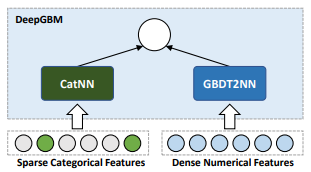
Figure 1: The framework of DeepGBM, which consists of two components, CatNN and GBDT2NN, to handle the sparse categorical and dense numerical features, respectively.

DeepGBM의 프레임워크는 CatNN과 GBDT2NN의 두 가지 구성 요소로 구성되어 있으며, 각각 희박한 고양이 등극 및 고밀도 수치 특징을 처리한다.

Data Mining (KDD ’19), August 4–8, 2019, Anchorage, AK, USA. ACM, New York, NY, USA, 11 pages.

https://doi.org/10.1145/3292500.3330858

1. INTRODUCTION

Online prediction represents a certain type of tasks playing the essential role in many real-world industrial applications, such as click prediction [21, 22, 36, 51] in sponsored search, content ranking [1, 6, 7] in Web search, content optimization [9, 10, 47] in recommender systems, travel time estimation [31, 49] in transportation planning, etc.

온라인 예측은 클릭 예측 [21, 22, 36, 51], 웹 검색의 콘텐츠 순위 [1, 6, 7], 리컴 벤더 시스템의 콘텐츠 최적화 [9, 10, 47], 이동 시간 추정 [31, 49]과 같은 많은 실제 산업 애플리케이션에서 필수적인 역할을 하는 특정 유형의 작업을 나타낸다.

A typical online prediction task usually yields two specific characteristics in terms of the tabular input space and the online data generation.

일반적인 온라인 예측 작업은 일반적으로 표 입력 공간과 온라인 데이터 생성 측면에서 두 가지 특정 특성을 산출한다.

In particular, the tabular input space means that the input features of an online prediction task can include both categorical and numerical tabular features.

특히, 표 입력 공간은 온라인 예측 작업의 입력 기능이 범주형 및 숫자형 특징을 모두 포함할 수 있음을 의미한다.

For example, the feature space of the click prediction task in sponsored search usually contains categorical ones like the ad category as well as numerical ones like the textual similarity between the query and the ad.

예를 들어, 후원 검색에서 클릭 예측 작업의 특징 공간은 일반적으로 쿼리와 광고 사이의 텍스트 유사성과 같은 숫자 범주뿐만 아니라 광고 범주와 같은 범주형도 포함한다.

In the meantime, the online data generation implies that the real data of those tasks are generated in the online mode and the data distribution could be dynamic in real time.

한편, 온라인 데이터 생성은 이러한 작업의 실제 데이터가 온라인 모드에서 생성되고 데이터 배포가 실시간으로 동적일 수 있음을 암시한다.

For instance, the news recommender system can generate a massive amount of data in real time, and the ceaseless emerging news could give rise to dynamic feature distribution at a different time.

예를 들어, 뉴스 추천자 시스템은 엄청난 양의 데이터를 실시간으로 생성할 수 있으며, 끊임없이 등장하는 뉴스는 다른 시간에 동적 기능 배포를 발생시킬 수 있습니다.

Therefore, to pursue an effective learning-based model for the online prediction tasks, it becomes a necessity to address two main challenges:

따라서 온라인 예측 과제에 대한 효과적인 학습 기반 모델을 추구하기 위해서는 다음과 같은 두 가지 주요 과제를 해결해야 한다.

(1) how to learn an effective model with tabular input space; and

표 형식 입력 공간을 사용하여 효과적인 모델을 학습하는 방법.

(2) how to adapt the model to the online data generation.

온라인 데이터 생성에 맞게 모델을 조정하는 방법

Currently, two types of machine learning models are widely used to solve online prediction tasks, i.e., Gradient Boosting Decision Tree (GBDT) and Neural Network (NN)1 .

현재 온라인 예측 작업을 해결하는 데 널리 사용되는 두 가지 유형의 기계 학습 모델, 즉 GBDT(Gradient Boosting Decision Tree)와 신경망(NN)1이 있다.

Unfortunately, neither of them can simultaneously address both of those two main challenges well. In other words, either GBDT or NN yields its own pros and cons when being used to solve the online prediction tasks.

안타깝게도 두 가지 주요 과제를 동시에 해결할 수는 없습니다. 다시 말해, 온라인 예측 작업을 해결하는 데 사용할 때 GBDT 또는 NN 중 하나가 장단점을 산출한다.

On one side, GBDT’s main advantage lies in its capability in handling dense numerical features effectively.

한편으로 GBDT의 주요 장점은 고밀도 수치 특징을 효과적으로 처리할 수 있는 능력에 있다.

Since it can iteratively pick the features with the largest statistical information gain to build the trees [20, 45], GBDT can automatically choose and combine the useful numerical features to fit the training targets well 2.

트리를 구축하기 위해 통계 정보 이득이 가장 큰 특징을 반복적으로 선택할 수 있기 때문에 GBDT는 훈련 목표에 잘 맞도록 유용한 수치 특징을 자동으로 선택하고 결합할 수 있다.

That is why GBDT has demonstrated its effectiveness in click prediction [33], web search ranking [6], and other well-recognized prediction tasks [8].

그렇기 때문에 GBDT는 클릭 예측[33], 웹 검색 순위[6] 및 기타 잘 알려진 예측 작업에서 그 효과를 입증했다[8].

Meanwhile, GBDT has two main weaknesses in online prediction tasks.

한편, GBDT는 온라인 예측 작업에서 두 가지 주요 약점을 가지고 있다.

First, as the learned trees in GBDT are not differentiable, it is hard to update the GBDT model in the online mode. Frequent retraining from scratch makes GBDT quite inefficient in learning over online prediction tasks.

첫째, GBDT에서 학습된 트리는 차별화할 수 없으므로 온라인 모드에서 GBDT 모델을 업데이트하기가 어렵다. 처음부터 재교육을 자주 하면 온라인 예측 작업에 대한 학습에서 GBDT가 상당히 비효율적이다.

This weakness, moreover, prevents GBDT from learning over very large scale data, since it is usually impractical to load a huge amount of data into the memory for learning 3.

게다가 이 약점은 GBDT가 대규모 데이터를 학습하는 것을 방해한다. 학습 3을 위해 메모리에 엄청난 양의 데이터를 로드하는 것은 일반적으로 비현실적이기 때문이다.

The second weakness of GBDT is its ineffectiveness in learning over sparse categorical features4 .

GBDT의 두 번째 약점은 희소 범주적 특징4에 대한 학습의 비효율성이다.

Particularly, after converting categorical features into sparse and high-dimensional one-hot encodings, the statistical information gain will become very small on sparse features, since the gain of imbalance partitions by sparse features is almost the same as non-partition.

특히 범주형 특징을 희소 및 고차원 단일 핫 코딩으로 변환한 후 희소 형상에 의한 불균형 파티션 이득이 비 파티션과 거의 같기 때문에 희소 형상에서 통계 정보 이득은 매우 작아진다.

As a result, GBDT fails to use sparse features to grow trees effectively.

따라서 GBDT는 희소 기능을 사용하여 트리를 효과적으로 성장시키지 못합니다.

Although there are some other categorical encoding methods [41] that can directly convert a categorical value into a dense numerical value, the raw information will be hurt in these methods as the encode values of different categories could be similar and thus we cannot distinguish them.

범주형 값을 조밀한 숫자 값으로 직접 변환할 수 있는 다른 범주형 인코딩 방법[41]이 있지만, 서로 다른 범주의 인코딩 값이 비슷할 수 있으므로 이러한 방법에서는 원시 정보가 손상될 수 있다.

Categorical features also could be directly used in tree learning, by enumerating possible binary partitions [16].

범주형 특성은 가능한 이진 파티션을 열거하여 트리 학습에도 직접 사용될 수 있다[16].

However, this method often overfits to the training data when with sparse categorical features, since there is too little data in each category and thus the statistical information is biased [29].

그러나 이 방법은 각 범주에 데이터가 너무 적어서 통계 정보가 편향되기 때문에 교리학적 특성이 희박한 경우 훈련 데이터에 과도하게 적합되는 경우가 많다[29].

In short, while GBDT can learn well over dense numerical features, the two weaknesses, i.e., the difficulty in adapting to online data generation and the ineffectiveness in learning over sparse categorical features, cause GBDT to fail in many online prediction tasks, especially those requiring the model being online adapted and those containing many sparse categorical features.

간단히 말해서, GBDT는 밀도가 높은 수치적 특징, 즉 온라인 데이터 생성에 적응하는 어려움과 희박한 범주적 특징에 대한 학습의 비효과적인 두 가지 약점은 많은 온라인 예측 작업, 특히 모델이 온라인에 적용되고 사람이 포함된 작업에서 GBDT가 실패하게 한다.y 희소 범주형 특성.

On the other side, NN’s advantages consist of its efficient learning over large scale data in online tasks since the batch-mode backpropagation algorithm as well as its capability in learning over sparse categorical features by the well-recognized embedding structure [35, 38].

반면에 NN의 장점은 배치 모드 역 전파 알고리즘 이후 온라인 작업에서 대규모 데이터에 대한 효율적인 학습과 잘 알려진 내장 구조에 의한 희소 범주적 특징에 대한 학습 능력[35, 38]으로 구성된다.

Some recent studies have revealed the success of employing NN in those online prediction tasks, including click prediction [22, 36, 51] and recommender systems [9, 10, 32, 38, 47].

클릭 예측 [22, 36, 51] 및 추천자 시스템 [9, 10, 32, 38, 47]을 포함하여 온라인 예측 작업에서 NN을 채택하는 데 성공했음을 일부 최근 연구에서 밝혀냈다.

Nevertheless, the main challenge of NN lies in its weakness in learning over dense numerical tabular features.

그럼에도 불구하고 NN의 주요 과제는 밀도가 높은 수치 표 형상에 대한 학습의 약점에 있다.

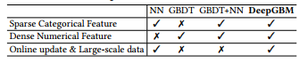
Table 1: Comparison over different models

표 1: 여러 모델에 대한 비교

Although a Fully Connected Neural Network (FCNN) could be used for dense numerical features directly, it usually leads to unsatisfactory performance, because its fully connected model structure leads to very complex optimization hyper-planes with a high risk of falling into local optimums [15].

완전 연결 신경망(FCNN)은 밀도가 높은 수치 형상에 직접 사용될 수 있지만, 완전 연결 모델 구조는 국부 최적값으로 떨어질 위험이 높은 매우 복잡한 최적화 초평면으로 이어지기 때문에 대개 만족스럽지 못한 성능을 초래한다[15].

Thus, in many tasks with dense numerical tabular features, NN often cannot outperform GBDT [8].

따라서 밀도가 높은 표 형상이 있는 많은 작업에서 NN은 종종 GBDT[8]를 능가할 수 없다.

To sum up, despite NN can effectively handle sparse categorical features and be adapted to online data generation efficiently, it is still difficult to result in an effective model by learning over dense numerical tabular features.

요약하자면, NN은 희소 범주적 특징을 효과적으로 처리하고 온라인 데이터 생성에 효율적으로 적응할 수 있지만, 밀도가 높은 수치 표 형상에 대해 학습하여 효과적인 모델을 도출하기는 여전히 어렵다.

As summarized in Table 1, either NN or GBDT yields its own pros and cons for obtaining the model for online prediction tasks.

표 1에 요약된 바와 같이, NN 또는 GBDT는 온라인 예측 작업에 대한 모델을 획득하는 데 자체적인 장단점을 산출한다.

Intuitively, it will be quite beneficial to explore how to combine the advantages of both NN and GBDT together, to address the two major challenges in online prediction tasks, i.e., tabular input space and online data generation, simultaneously.

직관적으로, 온라인 예측 작업, 즉 표 입력 공간과 온라인 데이터 생성의 두 가지 주요 과제를 동시에 해결하기 위해 NN과 GBDT의 장점을 결합하는 방법을 탐구하는 것이 매우 유익할 것이다.

In this paper, we propose a new learning framework, DeepGBM, which integrates NN and GBDT together, to obtain a more effective model for generic online prediction tasks.

본 논문에서 우리는 일반적인 온라인 예측 작업에 보다 효과적인 모델을 얻기 위해 NN과 GBDT를 통합하는 새로운 학습 프레임워크인 DeepGBM을 제안한다.

In particular, the whole DeepGBM framework, as shown in Fig. 1, consists of two major components: CatNN being an NN structure with the input of categorical features and GBDT2NN being another NN structure with the input of numerical features.

특히, 그림 1에 나타난 바와 같이 전체 DeepGBM 프레임워크는 두 가지 주요 구성 요소로 구성된다. CatNN은 범주형 형상의 입력이 있는 NN 구조이고 GBDT2NN은 수치 형상의 입력이 있는 또 다른 NN 구조이다.

To take advantage of GBDT’s strength in learning over numerical features, GBDT2NN attempts to distill the knowledge learned by GBDT into an NN modeling process.

수치적 특징을 학습하는 GBDT의 강점을 이용하기 위해 GBDT2NN은 GBDT가 학습한 지식을 NN 모델링 프로세스로 증류하려고 한다.

Specifically, to boost the effectiveness of knowledge distillation [24], GBDT2NN does not only transfer the output knowledge of the pre-trained GBDT but also incorporates the knowledge of both feature importance and data partition implied by tree structures from obtained trees.

특히, 지식 증류[24]의 효과를 높이기 위해 GBDT2NN은 사전 훈련된 GBDT의 출력 지식을 전달할 뿐만 아니라 획득한 트리의 트리 구조에 의해 암시되는 기능 중요성과 데이터 파티션에 대한 지식을 통합한다.

In this way, in the meantime achieving the comparable performance with GBDT, GBDT2NN, with the NN structure, can be easily updated by continuous emerging data when facing the online data generation.

이러한 방식으로 GBDT와 유사한 성능을 달성하는 한편, NN 구조를 가진 GBDT2NN은 온라인 데이터 생성에 직면할 때 지속적으로 등장하는 데이터를 통해 쉽게 업데이트할 수 있다.

Powered by two NN based components, CatNN and GBDT2NN, DeepGBM can indeed yield strong learning capacity over both categorical and numerical features while retaining the vital ability of efficient online learning.

CatNN과 GBDT2NN이라는 두 NN 기반 구성요소로 구동되는 DeepGBM은 효율적인 온라인 학습의 중요한 능력을 유지하면서 범주 및 수치적 특징 모두에 대해 강력한 학습 용량을 제공할 수 있다.

To illustrate the effectiveness of the proposed DeepGBM, we conduct extensive experiments on various publicly available datasets with tabular data. Comprehensive experimental results demonstrate that DeepGBM can outperform other solutions in various prediction tasks.

제안된 DeepGBM의 효과를 설명하기 위해 표 형식의 데이터를 사용하여 공개적으로 사용할 수 있는 다양한 데이터 세트에 대해 광범위한 실험을 수행한다. 종합적인 실험 결과는 DeepGBM이 다양한 예측 작업에서 다른 솔루션을 능가할 수 있음을 보여준다.

In summary, the contributions of this paper are multi-fold:

요약하면, 본 논문의 기여는 여러 배이다.

• We propose DeepGBM to leverage both categorical and numerical features while retaining the ability of efficient online update, for all kinds of prediction tasks with tabular data, by combining the advantages of GBDT and NN.

  우리는 GBDT와 NN의 장점을 결합하여 모든 종류의 예측 작업에 대해 효율적인 온라인 업데이트 기능을 유지하면서 범주 및 수치 기능을 모두 활용할 것을 DeepGBM을 제안한다.

• We propose an effective solution to distill the learned knowledge of a GBDT model into an NN model, by considering the selected inputs, structures and outputs knowledge in the learned tree of GBDT model.

  GBDT 모델의 학습 트리에서 선택한 입력, 구조 및 출력 지식을 고려하여 GBDT 모델의 학습된 지식을 NN 모델로 증류하는 효과적인 솔루션을 제안한다.

• Extensive experiments show that DeepGBM is an off-the-shelf model, which can be ready to use in all kinds of prediction tasks and achieves state-of-the-art performance.

  광범위한 실험에 따르면 DeepGBM은 모든 종류의 예측 작업에 사용할 수 있고 최첨단 성능을 달성할 수 있는 기성 모델입니다.

2. RELATED WORK

As aforementioned, both GBDT and NN have been widely used to learn the models for online prediction tasks.

앞서 언급한 것처럼 GBDT와 NN은 온라인 예측 작업의 모델을 학습하는 데 널리 사용되어 왔다.

Nonetheless, either of them yields respective weaknesses when facing the tabular input space and online data generation.

그럼에도 불구하고 표 형식 입력 공간과 온라인 데이터 생성에 직면할 때 이들 중 어느 쪽이든 각각의 약점을 산출한다.

In the following of this section, we will briefly review the related work in addressing the respective weaknesses of either GBDT or NN, followed by previous efforts that explored to combine the advantages of GBDT and NN to build a more effective model for online prediction tasks.

이 절의 다음 부분에서는 GBDT 또는 NN의 각각의 약점을 해결하는 관련 작업을 간략히 검토한 후 온라인 예측 작업에 보다 효과적인 모델을 구축하기 위해 GBDT와 NN의 장점을 결합하기 위한 이전의 노력을 검토한다.

2.1 Applying GBDT for Online Prediction Tasks

Applying GBDT for online prediction tasks yields two main weaknesses.

온라인 예측 작업에 GBDT를 적용하면 두 가지 주요 약점이 발생한다.

First, the non-differentiable nature of trees makes it hard to update the model in the online mode.

첫째, 트리의 차별화 불가능한 특성으로 인해 온라인 모드에서 모델을 업데이트하기가 어렵다.

Additionally, GBDT fails to effectively leverage sparse categorical features to grow trees.

또한 GBDT는 희소 범주 기능을 효과적으로 활용하여 트리를 성장시키지 못한다.

There are some related works that tried to address these problems.

이러한 문제를 해결하기 위해 노력한 관련 연구들이 있다.

Online Update in Trees.

트리의 온라인 업데이트.

Some studies have tried to train tree based models from streaming data [4, 11, 18, 28], however, they are specifically designed for the single tree model or multiple parallel trees without dependency, like Random Forest [3], and are not easy to apply to GBDT directly.

일부 연구에서는 스트리밍 데이터[4, 11, 18, 28]에서 트리 기반 모델을 훈련시키려고 시도했지만, 랜덤 포레스트[3]와 같이 단일 트리 모델 또는 종속성이 없는 다중 병렬 트리를 위해 특별히 설계되었으며 GBDT에 직접 적용하기가 쉽지 않다.

Moreover, they can hardly perform better than learning from all data at once.

또한, 한 번에 모든 데이터에서 학습하는 것보다 더 나은 성능을 발휘하기는 어렵다.

Two well-recognized open-sourced tools for GBDT, i.e., XGBoost [8] and LightGBM [29], also provide a simple solution for updating trees by online generated data.

GBDT에 대해 잘 알려진 두 개의 오픈 소스 툴(예: XGBoost[8] 및 LightGBM[29])도 온라인 생성 데이터에 의한 트리 업데이트를 위한 간단한 솔루션을 제공합니다.

In particular, they keep the tree structures fixed and update the leaf outputs by the new data. However, this solution can cause performance far below satisfaction.

특히, 그들은 트리 구조를 고정시키고 새로운 데이터로 리프 출력을 업데이트한다. 그러나 이 솔루션은 만족도에 훨씬 못 미치는 성능을 유발할 수 있습니다.

Further efforts Son et al. [44] attempted to re-find the split points on tree nodes only by the newly generated data.

Son 등[44]은 추가로 새로 생성된 데이터만으로 트리 노드에서 분할점을 다시 찾으려고 시도했다.

But, as such a solution abandons the statistical information over historical data, the split points found by the new data is biased and thus the performance is unstable.

그러나 이러한 솔루션은 과거 데이터에 대한 통계 정보를 포기하므로 새 데이터에 의해 발견된 분할점이 편향되어 성능이 불안정합니다.

Categorical Features in Trees.

트리의 범주 특성.

Since the extremely sparse and high-dimensional features, representing high cardinality categories, may cause very small statistical information gain from imbalance partitions, GBDT cannot effectively use sparse features to grow trees.

높은 카디널리티 범주를 나타내는 극도로 희박하고 고차원적인 특징은 불균형 파티션에서 매우 작은 통계 정보 이득을 야기할 수 있기 때문에 GBDT는 희소 특징을 효과적으로 사용하여 트리를 성장시킬 수 없다.

Some other encoding methods [41] tried to convert a categorical value into a dense numerical value such that they can be well handled by decision trees. CatBoost [12] also used the similar numerical encoding solution for categorical features.

일부 다른 인코딩 방법[41]은 의사결정 트리가 잘 처리할 수 있도록 범주형 값을 고밀도 숫자 값으로 변환하려고 시도했다. CatBoost[12]도 범주형 특징에 유사한 숫자 인코딩 솔루션을 사용했습니다.

However, it will cause information loss. Categorical features also could be directly used in tree learning, by enumerating possible binary partitions [16].

하지만, 그것은 정보 손실을 일으킬 것이다. 범주형 특성은 가능한 이진 파티션을 열거하여 트리 학습에도 직접 사용될 수 있다[16].

However, this method often over-fits to the training data when with sparse categorical features, since there is too little data in each category and thus the statistical information is biased [29].

그러나 이 방법은 각 범주에 데이터가 너무 적어서 통계 정보가 편향되기 때문에 범주적 특성이 희박한 경우 훈련 데이터에 과도하게 적합되는 경우가 많다[29].

There are some other works, such as DeepForest [52] and mGBDT [14], that use trees as building blocks to build multi-layered trees.

DeepForest[52]와 mGBDT[14]와 같은 다른 작품들도 있습니다. 나무를 빌딩 블록으로 사용하여 다층 트리를 만드는 것입니다.

However, they cannot be employed to address either the challenge of online update or that of learning over the categorical feature.

그러나 온라인 업데이트 또는 범주적 기능에 대한 학습 과제를 해결하기 위해 이러한 기능을 사용할 수는 없다.

In a word, while there were continuous efforts in applying GBDT to online prediction tasks, most of them cannot effectively address the critical challenges in terms of how to handle online data generation and how to learn over categorical features.

한마디로, 온라인 예측 작업에 GBDT를 적용하는 지속적인 노력이 있었지만, 대부분은 온라인 데이터 생성 처리 방법과 범주형 특징에 대한 학습 방법 측면에서 중요한 과제를 효과적으로 해결할 수 없다.

2.2 Applying NN for Online Prediction Tasks

온라인 예측 작업에 NN 적용

Applying NN for online prediction tasks yields one crucial challenge, i.e. NN cannot learn effectively over the dense numerical features.

온라인 예측 작업에 NN을 적용하면 한 가지 중요한 과제가 발생한다. 즉, NN은 밀도가 높은 수치 특징을 효과적으로 학습할 수 없다.

Although there are many recent works that have employed NN into prediction tasks, such as click prediction [22, 36, 51] and recommender systems [9, 10, 32, 47], they all mainly focused on the sparse categorical features, and far less attention has been put on adopting NN over dense numerical features, which yet remains quite challenging.

클릭 예측[22, 36, 51] 및 추천자 시스템[9, 10, 32, 47]과 같은 예측 작업에 NN을 채택한 많은 최근 연구가 있지만, 이들은 모두 희박한 범주적 특징에 초점을 맞췄고, 아직까지는 상당히 어려운 고밀도 수치 특징에 비해 NN 채택에 훨씬 덜 주의를 기울였다.

Traditionally, Fully Connected Neural Network (FCNN) is often used for dense numerical features.

전통적으로 FCNN(Fully Connected Neural Network)은 종종 고밀도 수치 형상에 사용된다.

Nevertheless, FCNN usually fails to reach satisfactory performance [15], because its fully connected model structure leads to very complex optimization hyper-planes with a high risk of falling into local optimums. Even after employing the certain normalization [27] and regularization [43] techniques, FCNN still cannot outperform GBDT in many tasks with dense numerical features [8].

그럼에도 불구하고 FCNN은 완전히 연결된 모델 구조가 로컬 최적에 빠질 위험이 높은 매우 복잡한 최적화 하이퍼 평면으로 이어지기 때문에 대개 만족스러운 성능에 도달하지 못한다[15]. 특정 정규화[27] 및 정규화[43] 기법을 사용한 후에도 FCNN은 여전히 밀도가 높은 수치 특징을 가진 많은 작업에서 GBDT를 능가할 수 없다[8].

Another widely used solution facing dense numerical features is discretization [13], which can bucketize numerical features into categorical formats and thus can be better handled by previous works on categorical features.

밀도가 높은 수치 형상에 직면하는 또 다른 널리 사용되는 솔루션은 이산화[13]로, 수치 형상을 범주형 형식으로 버킷화할 수 있으므로 범주형 형상에 대한 이전 연구에서 더 잘 처리할 수 있다.

However, since the bucketized outputs will still connect to fully connected layers, discretization actually cannot improve the effectiveness in handling numerical features.

그러나 버킷화된 출력은 여전히 완전히 연결된 레이어에 연결되기 때문에 이산화는 실제로 수치 형상의 처리 효과를 향상시킬 수 없다.

And discretization will increase the model complexity and may cause over-fitting due to the increase of model parameters.

또한 이산화는 모델 복잡성을 증가시키고 모델 매개변수의 증가로 인해 과적합을 유발할 수 있다.

To summarize, applying NN to online prediction tasks still suffers from the incapability in learning an effective model over dense numerical features.

요약하면, 온라인 예측 작업에 NN을 적용하는 것은 여전히 밀도가 높은 수치 특징에 대해 효과적인 모델을 학습할 수 없는 어려움을 겪고 있다.

2.3 Combining NN and GBDT

NN과 GBDT 결합

Due to the respective pros and cons of NN and GBDT, there have been emerging efforts that proposed to combine their advantages.

NN과 GBDT의 장단점 때문에 이들의 장점을 결합할 것을 제안하는 새로운 노력이 있었다.

In general, these efforts can be categorized into three classes:

일반적으로 이러한 노력은 세 가지 클래스로 분류될 수 있습니다.

Tree-like NN.

나무 같은 NN.

As pointed by Ioannou et al. [26], tree-like NNs, e.g. GoogLeNet [46], have decision ability like trees to some extent. There are some other works [30, 40] that introduce decision ability into NN.

Ioannou 등이 지적한 바와 같이. [26], 나무와 같은 NN(예: GoogLeNet[46])은 어느 정도 나무와 같은 의사 결정 능력을 가지고 있다. 의사 결정 능력을 NN에 도입하는 다른 작업[30, 40]도 있다.

However, these works mainly focused on computer vision tasks without attention to online prediction tasks with tabular input space. Yang et al. [50] proposed the soft binning function to simulate decision trees in NN, which is, however, very inefficient as it enumerates all possible decisions. Wang et al. [48] proposed NNRF, which used tree-like NN and random feature selection to improve the learning from tabular data.

그러나 이러한 작업은 표 입력 공간이 있는 온라인 예측 작업에 주의를 기울이지 않고 주로 컴퓨터 비전 작업에 초점을 맞췄다. 양 외 연구진 [50]은 NN에서 의사 결정 트리를 시뮬레이션하기 위한 소프트 비닝 함수를 제안했지만, 가능한 모든 의사 결정을 열거하기 때문에 매우 비효율적이다. 왕 외 연구진 [48] 표 형식 데이터에서 학습을 개선하기 위해 트리형 NN과 무작위 기능 선택을 사용한 NNRF를 제안했다.

Nevertheless, NNRF simply uses random feature combinations, without leveraging the statistical information over training data like GBDT.

그럼에도 불구하고 NNRF는 GBDT와 같은 훈련 데이터에 대한 통계 정보를 활용하지 않고 무작위의 기능 조합을 사용한다.

Convert Trees to NN.

트리를 NN으로 변환합니다.

Another track of works tried to convert the trained decision trees to NN [2, 5, 25, 39, 42].

다른 작업 트랙은 훈련된 의사 결정 트리를 NN[2, 5, 25, 39, 42]으로 변환하려고 시도했다.

However, these works are inefficient as they use a redundant and usually very sparse NN to represent a simple decision tree.

그러나 이러한 작업은 중복되고 대개 매우 희박한 NN을 사용하여 단순한 의사 결정 트리를 나타내기 때문에 비효율적이다.

When there are many trees, such conversion solution has to construct a very wide NN to represent them, which is unfortunately hard to be applied to realistic scenarios.

트리가 많은 경우 이러한 변환 솔루션은 트리를 나타내기 위해 매우 넓은 NN을 구성해야 하며, 이는 유감스럽게도 현실적인 시나리오에 적용되기 어렵다.

Furthermore, these methods use the complex rules to convert a single tree and thus are not easily used in practice.

또한 이러한 방법은 하나의 트리를 변환하기 위해 복잡한 규칙을 사용하므로 실제로 쉽게 사용되지 않습니다.

Combining NN and GBDT.

NN과 GBDT를 결합합니다.

There are some practical works that directly used GBDT and NN together [23, 33, 53].

GBDT와 NN을 직접 사용한 몇 가지 실제 작업이 있다[23, 33, 53].

Facebook [23] used the leaf index predictions as the input categorical features of a Logistic Regression.

Facebook [23]에서는 잎 지수 예측을 로지스틱 회귀 분석의 입력 범주형 특징으로 사용했습니다.

Microsoft [33] used GBDT to fit the residual errors of NN.

Microsoft [33]에서는 NN의 잔여 오류를 맞추기 위해 GBDT를 사용했습니다.

However, as the online update problem in GBDT is not resolved, these works cannot be efficiently used online.

그러나 GBDT의 온라인 업데이트 문제가 해결되지 않아 온라인에서 이러한 작업을 효율적으로 사용할 수 없습니다.

In fact, Facebook also pointed up this problem in their paper [23], for the GBDT model in their framework needs to be retrained every day to achieve the good online performance.

실제로 Facebook도 논문 [23]에서 이 문제를 지적했는데, 프레임워크의 GBDT 모델은 좋은 온라인 성능을 얻기 위해 매일 재교육을 받아야 한다.

As a summary, while there are increasing efforts that explored to combine the advantages of GBDT and NN to build a more effective model for online prediction tasks, most of them cannot totally address the challenges related to tabular input space and online data generation.

요약하자면, 온라인 예측 작업에 보다 효과적인 모델을 구축하기 위해 GBDT와 NN의 장점을 결합하려는 노력이 증가하고 있지만, 이들 대부분은 표 입력 공간 및 온라인 데이터 생성과 관련된 과제를 완전히 해결할 수 없다.

In this paper, we propose a new learning framework, DeepGBM, to better integrates NN and GBDT together.

본 논문에서 우리는 NN과 GBDT를 더 잘 통합하기 위한 새로운 학습 프레임워크인 DeepGBM을 제안한다.

3. DEEPGBM

In this section, we will elaborate on how the new proposed learning framework, DeepGBM, integrates NN and GBDT together to obtain a more effective model for generic online prediction tasks.

이 절에서는 새로운 제안된 학습 프레임워크인 DeepGBM이 NN과 GBDT를 통합하여 일반적인 온라인 예측 작업에 보다 효과적인 모델을 얻는 방법에 대해 자세히 설명하겠다.

Specifically, the whole DeepGBM framework, as shown in Fig. 1, consists of two major components: CatNN being an NN structure with the input of categorical features and GBDT2NN being another NN structure distilled from GBDT with focusing on learning over dense numerical features.

구체적으로, 그림 1에 표시된 바와 같이 전체 DeepGBM 프레임워크는 두 가지 주요 구성 요소로 구성된다. CatNN은 범주형 특징을 입력하는 NN 구조이고 GBDT2NN은 고밀도 수치 특징을 학습하는 데 초점을 맞춘 GBDT에서 증류된 또 다른 NN 구조이다.

We will describe the details of each component in the following subsections.

각 구성 요소의 세부 사항은 다음 하위 절에서 설명하겠습니다.

3.1 CatNN for Sparse Categorical Features

희소 범주형 특징을 위한 CatNN

To solve online prediction tasks, NN has been widely employed to learn the prediction model over categorical features, such as Wide & Deep [9], PNN [36], DeepFM [22] and xDeepFM [32].

온라인 예측 작업을 해결하기 위해 NN은 Wide & Deep [9], PNN [36], DeepFM [22] 및 xDeep과 같은 범주적 기능에 대한 예측 모델을 학습하기 위해 널리 사용되어 왔다.FM [32].

Since the target of CatNN is the same as these works, we can directly leverage any of existing successful NN structures to play as the CatNN, without reinventing the wheel.

CatNN의 대상이 이러한 작업과 동일하기 때문에, 우리는 바퀴를 재창조하지 않고도 기존의 성공적인 NN 구조를 CatNN으로 플레이하기 위해 직접 활용할 수 있다.

In particular, the same as previous works, CatNN mainly relies on the embedding technology, which can effectively convert the high dimensional sparse vectors into dense ones.

특히 이전 작업과 마찬가지로 CatNN은 고차원 희소 벡터를 고밀도 벡터로 효과적으로 변환할 수 있는 임베딩 기술에 주로 의존한다.

Besides, in this paper, we also leverage FM component and Deep component from previous works [9, 22], to learn the interactions over features. Please note CatNN is not limited by these two components, since it can use any other NN components with similar functions.

또한 본 논문에서는 이전 작업[9, 22]의 FM 구성 요소와 Deep 구성 요소를 활용하여 특징에 대한 상호 작용을 학습한다. CatNN은 유사한 기능을 가진 다른 NN 구성 요소를 사용할 수 있으므로 이 두 구성 요소에 의해 제한되지 않습니다.

Embedding is the low-dimensional dense representation of a high-dimensional sparse vector, and can denote as

임베딩은 고차원 희소 벡터의 저차원 밀도 표현이며 다음과 같이 나타낼 수 있다.

where xi is the value of i -th feature, Vi stores all embeddings of the i th feature and can be learned by back-propagation, and EVi (xi ) will return the corresponding embedding vector for xi .

여기서 xi는 i -th 형상의 값이며 Vi는 i th 형상의 모든 임베딩을 저장하고 역전파를 통해 학습할 수 있으며 EVi(xi )는 xi 에 해당하는 임베딩 벡터를 반환합니다.

Based on that, we can use FM component to learn linear (order-1) and pair-wise (order-2) feature interactions, and denote as

이를 바탕으로 FM 구성요소를 사용하여 선형(차수-1) 및 쌍방향(차수-2) 특징 상호작용을 학습할 수 있으며, 다음과 같이 나타낼 수 있다.

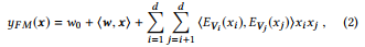
where d is the number of features, w0 and w are the parameters of linear part, and ⟨·, ·⟩ is the inner product operation.

여기서 d는 형상의 수이고, w0과 w는 선형 부품의 매개변수이며, ··, ·d는 내부 제품 연산이다.

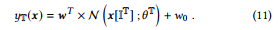
Then, Deep component is used to learn the high-order feature interactions:

그런 다음 Deep 구성 요소를 사용하여 고차 기능 상호 작용을 학습합니다.

where N (x ; θ ) is a multi-layered NN model with input x and parameter θ.

여기서 N(x; θ )은 입력 x와 파라미터 . 를 가진 다중 레이어 NN 모델이다.

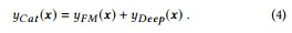
Combined with two components, the final output of CatNN is

CatNN의 최종 출력은 다음과 같다.

3.2 GBDT2NN for Dense Numerical Features

고밀도 수치 특징을 위한 GBDT2NN

In this subsection, we will describe the details about how we distill the learned trees in GBDT into an NN model.

이 하위 절에서는 GBDT에서 학습된 트리를 NN 모델로 증류하는 방법에 대한 세부 정보를 설명한다.

Firstly, we will introduce how to distill a single tree into an NN.

먼저 단일 트리를 NN으로 증류하는 방법을 소개한다.

Then, we will generalize the idea to the distillation from multiple trees in GBDT.

그런 다음 GBDT의 여러 나무에서 추출하여 아이디어를 일반화합니다.

3.2.1

Single Tree Distillation.

단일 트리 증류.

Most of the previous distillation works only transfer model knowledge in terms of the learned function, in order to ensure the new model generates a similar output compared to the transferred one.

대부분의 이전 증류는 학습된 함수 측면에서 모델 지식만 전송하여 새 모델이 전송된 모델과 유사한 출력을 생성하도록 한다.

However, since tree and NN are naturally different, beyond traditional model distillation, there is more knowledge in the tree model could be distilled and transferred into NN.

그러나 트리와 NN은 기존 모델 증류를 넘어 자연적으로 다르기 때문에 트리 모델에 더 많은 지식이 증류되어 NN으로 전달될 수 있다.

In particular, the feature selection and importance in learned trees, as well as data partition implied by learned tree structures, are indeed other types of important knowledge in trees.

특히 학습된 나무 구조에 의해 암시되는 데이터 파티션뿐만 아니라 학습된 나무의 특징 선택과 중요성은 실제로 나무의 다른 유형의 중요한 지식이다.

Tree-Selected Features.

트리가 선택한 기능.

Compared to NN, a special characteristic of the tree-based model is that it may not use all input features, as its learning will greedily choose the useful features to fit the training targets, based on the statistical information.

NN과 비교하여 트리 기반 모델의 특별한 특징은 학습이 통계 정보를 기반으로 훈련 목표에 맞는 유용한 특징을 탐욕스럽게 선택하기 때문에 모든 입력 기능을 사용하지 않을 수 있다는 것이다.

Therefore, we can transfer such knowledge in terms of tree-selected features to improve the learning efficiency of the NN model, rather than using all input features.

따라서 모든 입력 기능을 사용하는 대신 NN 모델의 학습 효율성을 개선하기 위해 트리 선택 기능 측면에서 이러한 지식을 전달할 수 있다.

In particular, we can merely use the tree-selected features as the inputs of NN.

특히 트리 선택 기능을 NN의 입력으로 사용할 수 있다.

Formally, we define It as the indices of the used features in a tree t.

공식적으로, 우리는 그것을 트리 t에서 사용된 형상의 지수로 정의한다.

Then we can only use x [It ] as the input of NN.

그러면 NN의 입력으로 x [It]만 사용할 수 있습니다.

Tree Structure.

트리 구조.

Essentially, the knowledge of tree structure of a decision tree indicates how to partition data into many nonoverlapping regions (leaves), i.e., it clusters data into different classes and the data in the same leaf belongs to the same class.

기본적으로 의사 결정 트리의 트리 구조에 대한 지식은 데이터를 중복되지 않는 많은 영역(리브)으로 분할하는 방법을 나타냅니다. 즉, 데이터를 다른 클래스로 클러스터링하고 동일한 리프의 데이터는 동일한 클래스에 속합니다.

It is not easy to directly transfer such tree structure into NN, as their structures are naturally different.

이러한 트리 구조를 NN으로 직접 전송하는 것은 쉽지 않다. 그 구조는 본질적으로 다르기 때문이다.

Fortunately, as NN has been proven powerful enough to approximate any functions [19], we can use an NN model to approximate the function of the tree structure and achieve the structure knowledge distillation.

다행히도, NN은 모든 기능에 근사할 만큼 충분히 강력하다는 것이 입증되었기 때문에, 우리는 NN 모델을 사용하여 트리 구조의 기능을 근사화하고 구조 지식 증류를 달성할 수 있다.

Therefore, as illustrated in Fig.2, we can use NN to fit the cluster results produced by the tree, to let NN approximate the structure function of decision tree.

따라서 그림 2에서 설명한 것처럼 NN을 사용하여 트리에서 생성된 클러스터 결과를 적합시켜 NN이 의사 결정 트리의 구조 기능을 근사하게 만들 수 있다.

Formally, we denote the structure function of a tree t as Ct (x ), which returns the output leaf index, i.e. the cluster result produced by the tree, of sample x .

공식적으로, 우리는 트리 t의 구조 함수를 Ct (x)로 나타내며, 이는 샘플 x의 출력 리프 색인, 즉 트리에 의해 생성된 클러스터 결과를 반환한다.

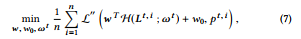
Then, we can use an NN model to approximate the structure function Ct (·) and the learning process can denote as

그런 다음 NN 모델을 사용하여 구조 함수 Ct (·)를 근사할 수 있으며 학습 과정은 다음과 같이 나타낼 수 있다.

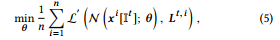
where n is the number of training samples, x i is the i -th training sample, Lt , i is the one-hot representation of leaf index Ct (x i ) for x i, It is the indices of used features in tree t , θ is the parameter of NN model N and can be updated by back-propagation, L is the loss function for the multiclass problem like cross entropy.

여기서 n은 훈련 샘플의 수, x i는 i번째 훈련 샘플, Lt , i는 x i에 대한 잎 지수 Ct (x i )의 원핫 표현, 이는 트리 t에서 사용된 형상의 지수이며 is는 NN 모델 N의 매개 변수이며 교차 엔트로피와 같은 다중 클래스 문제에 대한 손실 함수이다.

Thus, after learning, we can get an NN model N (· ; θ ). Due to the strong expressiveness ability of NN, the learned NN model should perfectly approximate the structure function of decision tree.

따라서 학습 후 NN 모델 N(· ; ). )을 얻을 수 있다. NN의 강력한 표현 능력 때문에, 학습된 NN 모델은 의사결정 트리의 구조 기능과 완벽하게 유사해야 한다.

Tree Outputs.

트리 출력.

Since the mapping from tree inputs to tree structures is learned in the previous step, to distill tree outputs, we only need to know the mapping from tree structures to tree outputs.

트리 입력에서 트리 구조로의 매핑은 이전 단계에서 학습되었으므로 트리 출력을 증류하려면 트리 구조에서 트리 출력으로의 매핑만 알면 된다.

As there is a corresponding leaf value for a leaf index, this mapping is actually not needed to learn.

리프 인덱스에 해당하는 리프 값이 있으므로 이 매핑은 실제로 학습에 필요하지 않습니다.

In particular, we denote the leaf values of tree t as qt and qit represents the leaf value of i-th leaf.

특히 qt와 qit는 i-th leaf의 잎 값을 나타내므로 트리 t의 잎 값을 나타낸다.

Then we can map Lt to the tree output by pt = Lt × qt.

그러면 우리는 pt = Lt × qt로 Lt를 트리 출력에 매핑할 수 있다.

Combined with the above methods for single tree distillation, the output of NN distilled from tree t can denote as

단일 트리 증류를 위한 위의 방법과 결합하여, 트리 t에서 증류된 NN의 출력은 다음과 같이 나타낼 수 있다.

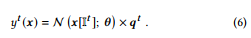
Figure 2: Tree structure distillation by leaf index. NN will approximate the tree structure by fitting its leaf index.

그림 2: 잎 지수에 의한 나무 구조 증류. NN은 리프 인덱스를 맞춤으로써 트리 구조의 근사치를 구한다.

Figure 3: Tree structure distillation by leaf embedding.
The leaf index is first transformed to leaf embedding.
Then NN will approximate tree structure by fitting the leaf embedding.
Since the dimension of leaf embedding can be significantly smaller than the leaf index, this distillation method will be much more efficient.

그림 3: 잎을 내장하여 나무 구조를 증류합니다.
리프 인덱스는 먼저 리프 임베딩으로 변환됩니다.
그런 다음 NN은 리프 임베딩에 적합하여 트리 구조를 근사화한다.
잎 내장 치수는 잎 지수보다 상당히 작을 수 있기 때문에, 이 증류 방법은 훨씬 더 효율적일 것이다.

3.2.2

Multiple Tree Distillation.

Since there are multiple trees in GBDT, we should generalize the distillation solution for the multiple trees.

GBDT에는 여러 트리가 있으므로 여러 트리의 증류액을 일반화해야 합니다.

A straight-forward solution is using #NN = #tree NN models, each of them distilled from one tree.

간단한 해결책은 #N N = #tree NN 모델을 사용하는 것이며, 각 모델은 하나의 트리에서 증류된다.

However, this solution is very inefficient due to the high dimension of structure distillation targets, which is O(|L| ×#NN ).

그러나, 이 용액은 O(|L| ×#NN)인 구조 증류 대상의 높은 차원 때문에 매우 비효율적이다.

To improve the efficiency, we propose Leaf Embedding Distillation and Tree Grouping to reduce |L| and #NN respectively.

효율성을 개선하기 위해 |L|과 #NN을 각각 줄이기 위한 리프 임베딩 증류 및 트리 그룹을 제안한다.

Leaf Embedding Distillation.

리프 내장 증류.

As illustrated in Fig.3, we adopt embedding technology to reduce the dimension of structure distillation targets L while retraining the information in this step.

그림 3에서 설명한 것처럼, 우리는 이 단계에서 정보를 재교육하면서 구조 증류 대상 L의 치수를 줄이기 위해 임베딩 기술을 채택한다.

More specifically, since there are bijection relations between leaf indices and leaf values, we use the leaf values to learn the embedding.

좀 더 구체적으로, 잎 지수와 잎 값 사이에는 상호 투영 관계가 있기 때문에, 우리는 잎 값을 사용하여 임베딩을 학습한다.

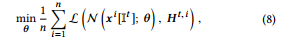
Formally, the learning process of embedding can denote as

공식적으로, 임베딩의 학습 과정은 다음과 같이 나타낼 수 있다.

where H t , i = H (Lt , i ; ωt ) is an one-layered fully connected network with parameter ωt that converts the one-hot leaf index Lt , i to the dense embedding H t , i , pt , i is the predict leaf value of sample x i, L ′′ is the same loss function as used in tree learning, w and w0 are the parameters for mapping embedding to leaf values.

여기서 H t , i = H (Lt , i ; tt )는 단일 핫 리프 지수 Lt , i를 밀집 임베딩 H t , i , pt 로 변환하는 매개변수 µt 를 가진 1개의 완전 연결 네트 작업이며, 표본 x i , i , pt 는 트리 학습에 사용되는 것과 동일한 리프 매핑의 손실 함수이다.

After that, instead of sparse high dimensional one-hot representation L, we can use the dense embedding as the targets to approximate the function of tree structure. This new learning process can denote as

그 후, 희박한 고차원 원핫 표현 L 대신, 고밀도 임베딩을 대상으로 사용하여 트리 구조의 기능을 근사화할 수 있다. 이 새로운 학습 과정은 다음과 같이 나타낼 수 있다.

where L is the regression loss like L2 loss for fitting dense embedding.

여기서 L은 조밀한 임베딩 장착을 위한 L2 손실과 같은 회귀 손실이다.

Since the dimension of H t , i should be much smaller than L, Leaf Embedding Distillation will be more efficient in the multiple tree distillation.

H t의 치수, i는 L보다 훨씬 작아야 하기 때문에, 잎 내장 증류는 다중 나무 증류에서 더 효율적일 것입니다.

Furthermore, it will use much fewer NN parameters and thus is more efficient.

또한 훨씬 적은 NN 매개변수를 사용하기 때문에 더 효율적이다.

Tree Grouping.

트리 그룹화.

To reduce the #N N , we can group the trees and use an NN model to distill from a group of trees.

#NN을 줄이기 위해 트리를 그룹화하고 NN 모델을 사용하여 트리 그룹에서 증류할 수 있다.

Subsequently, there are two problems for grouping:

이후 그룹화에는 두 가지 문제가 있습니다.

(1) how to group the trees and (2) how to distill from a group of trees.

(1) 나무를 그룹화하는 방법 및 (2) 나무 그룹에서 증류하는 방법

Firstly, for the grouping strategies, there are many solutions.

첫째, 그룹화 전략에는 많은 해결책이 있다.

For example, the equally randomly grouping, equally sequentially grouping, grouping based on importance or similarity, etc.

예를 들어, 균등 랜덤 그룹화, 균등 순차 그룹화, 중요도 또는 유사성을 기준으로 그룹화 등입니다.

In this paper, we use the equally randomly grouping.

이 문서에서는 균등하게 랜덤하게 그룹화하는 방법을 사용합니다.

Formally, assuming there are m trees and we want to divide them into k groups, there are s = ⌈m/k ⌉ trees in each group and the trees in j -th group are Tj , which contains random s trees from GBDT.

공식적으로, m개의 트리가 있고 그것들을 k개의 그룹으로 나누고 싶다고 가정하면, 각 그룹에는 s = µm/k ÷ 트리가 있고 j번째 그룹의 트리는 GBDT의 임의의 s 트리를 포함하는 Tj이다.

Secondly, to distill from multiple trees, we can extend the Leaf Embedding Distillation for multiple trees.

둘째, 여러 나무에서 증류하기 위해 여러 트리에 대한 잎 내장 증류를 확장할 수 있습니다.

Formally, given a group of trees T, we can extend the Eqn.(7) to learn leaf embedding from multiple trees

공식적으로, 나무 그룹 T가 주어지면, 우리는 Eqn.(7)을 확장하여 여러 나무에서 잎 임베딩을 배울 수 있다.

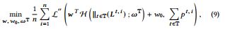
where ∥(·) is the concatenate operation, G T, i = H ∥t ∈T (Lt , i ) ; ωT is an one-layered fully connected network that convert the multihot vectors, which is the concatenate of multiple one-hot leaf index vectors, to a dense embedding G T, i for the trees in T.

여기서 (( · )는 연결 연산이고, G T, i = H tt tT (Lt, i ); tT는 다중 핫 벡터를 다중 핫 리프 인덱스 벡터의 결합인 고밀도 내장 G T로 변환하는 1개의 완전 연결 네트워크이다.

After that, we can use the new embedding as the distillation target of NN model, and the learning process of it can denote as

그 후에, 우리는 NN 모델의 증류 대상으로 새로운 임베딩을 사용할 수 있고, 그것의 학습 과정은 다음과 같이 나타낼 수 있다.

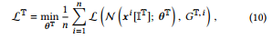
where IT is the used features in tree group T.

여기서 IT는 트리 그룹 T에서 사용되는 기능이다.

When the number of trees in T is large, IT may contains many features and thus hurt the feature selection ability.

T의 트리 수가 많은 경우 IT는 많은 기능을 포함하므로 기능 선택 기능에 손상을 줄 수 있습니다.

Therefore, as an alternate, we can only use top features in IT according to feature importance.

따라서 대신 기능 중요도에 따라 IT의 상위 기능만 사용할 수 있습니다.

To sum up, combined with above methods, the final output of the NN distilled from a tree group T is

위의 방법과 결합하면 트리 그룹 T에서 증류된 NN의 최종 출력은 다음과 같다.

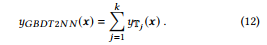
And the output of a GBDT model, which contains k tree groups, is

그리고 k개의 트리 그룹을 포함하는 GBDT 모델의 출력은

In summary, owing to Leaf Embedding Distillation and Tree Grouping, GBDT2NN can efficiently distill many trees of GBDT into a compact NN model.

요약하면, 잎 내장 증류 및 트리 그룹화로 인해 GBDT2NN은 GBDT의 많은 트리를 소형 NN 모델로 효율적으로 증류할 수 있다.

Furthermore, besides tree outputs, the feature selection and structure knowledge in trees are effectively distilled into the NN model as well.

또한 트리 출력 외에도 트리의 특징 선택과 구조 지식도 NN 모델로 효과적으로 증류된다.

3.3 Training for DeepGBM

DeepGBM 교육

We will describe how to train the DeepGBM in this subsection, including how to train it end-to-end offline and how to efficiently update it online.

우리는 이 하위섹션에서 DeepGBM을 오프라인으로 교육하는 방법과 온라인에서 효율적으로 업데이트하는 방법을 설명할 것이다.

3.3.1

End-to-End Offline Training.

단대단 오프라인 교육.

To train DeepGBM, we first need to use offline data to train a GBDT model and then use Eqn.(9) to get the leaf embedding for the trees in GBDT.

DeepGBM을 교육하려면 먼저 오프라인 데이터를 사용하여 GBDT 모델을 교육한 다음 Eqn.(9)을 사용하여 GBDT의 트리에 대한 리프 임베딩을 받아야 합니다.

After that, we can train DeepGBM end-to-end. Formally, we denote the output of DeepGBM as

그런 다음 DeepGBM을 처음부터 끝까지 교육할 수 있습니다. 공식적으로, 우리는 다음과 같이 DeepGBM의 출력을 나타낸다.

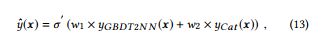
where w1 and w2 are the trainable parameters used for combining is GBDT2NN and CatNN, σ' is the output transformation, such as sigmoid for binary classification.

여기서 w1과 w2는 결합에 사용되는 훈련 가능한 파라미터이며, ''는 이진 분류를 위한 시그모이드와 같은 출력 변환이다.

Then, we can use the following loss function for the end-to-end training

그런 다음 다음 손실 함수를 엔드 투 엔드 교육에 사용할 수 있습니다.

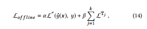
where y is the training target of sample x , L corresponding tasks such as cross-entropy for classification tasks, L T is the embedding loss for tree group T and defined in Eqn.(10), k is the number of tree groups, α and β are hyper-parameters given in advance and used for controlling the strength of end-to-end loss and embedding loss, respectively.

여기서 y는 분류 작업을 위한 교차 엔트로피와 같은 샘플 x , L 해당 작업의 훈련 대상이며, L T는 트리 그룹 T에 대한 내장 손실이며 Eqn(10), k는 트리 그룹 수, α 및 β는 미리 주어진 초 매개 변수이며 각각 엔드 투 엔드 손실 및 임베딩 손실의 강도를 제어하기 위해 사용된다..

3.3.2

Online Update.

온라인 업데이트.

As the GBDT model is trained offline, using it for embedding learning in the online update will hurt the online real-time performance.

GBDT 모델은 오프라인으로 교육되므로 온라인 업데이트에 학습을 포함시키는 데 사용할 경우 온라인 실시간 성능이 저하될 수 있습니다.

Thus, we do not include the LT in the online update, and the loss for the online update can denote as

따라서 온라인 업데이트에 LT를 포함하지 않으며, 온라인 업데이트의 손실은 다음과 같이 나타낼 수 있다.

which only uses the end-to-end loss. Thus, when using DeepGBM online, we only need the new data to update the model by L-online , without involving GBDT and retraining from scratch.

단대단 손실만 사용합니다. 따라서 DeepGBM을 온라인으로 사용할 경우 GBDT를 포함하고 처음부터 다시 교육하지 않고 L-online으로 모델을 업데이트하기 위해 새로운 데이터만 필요합니다.

In short, DeepGBM will be very efficient for online tasks.

간단히 말해서 DeepGBM은 온라인 작업에 매우 효율적일 것입니다.

Furthermore, it is also very effective since it can well handle both the dense numerical features and sparse categorical features.

또한 밀도가 높은 수치적 특징과 희박한 범주적 특징을 모두 잘 처리할 수 있기 때문에 매우 효과적이다.

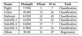
Table 2: Details of the datasets used in experiments. All these datasets are publicly available. #Sample is the number of data samples, #Num is the number of numerical features, and #Cat is the number of categorical features

표 2: 실험에 사용된 데이터 세트의 세부 정보. 이러한 모든 데이터 세트는 공개적으로 사용할 수 있습니다. #샘플은 데이터 샘플의 수, #Num은 숫자 형상의 수, #Cat은 범주 형상의 수입니다.

4. EXPERIMENT

실험

In this section, we will conduct thorough evaluations on DeepGBM5 over a couple of public tabular datasets and compares its performance with several widely used baseline models.

이 섹션에서는 몇 개의 공개 표 형식 데이터 세트에 대해 DeepGBM5에 대한 철저한 평가를 수행하고 그 성능을 널리 사용되는 여러 기준선 모델과 비교한다.

Particularly, we will start with details about experimental setup, including data description, compared models and some specific experiments settings.

특히, 데이터 설명, 비교 모델 및 일부 특정 실험 설정 등 실험 설정에 대한 세부 사항부터 시작하겠습니다.

After that, we will analyze the performance of DeepGBM in both offline and online settings to demonstrate its effectiveness and advantage over baseline models.

이후 오프라인 및 온라인 환경에서 DeepGBM의 성능을 분석하여 기준선 모델에 대한 효과와 이점을 입증할 것입니다.

4.1 Experimental Setup

실험 설정

Datasets: To illustrate the effective of DeepGBM, we conduct experiments on a couple of public datasets, as listed in Table 2.

Dataset: DeepGBM의 효과를 설명하기 위해 표 2에 나열된 것처럼 몇 개의 공개 데이터 세트에 대해 실험을 수행합니다.

In particular, Flight6 is an airline dataset and used to predict the flights are delayed or not. Criteo7, Malware8 and Zillow9 are the datasets from Kaggle competitions.

특히, Flight6는 항공사 데이터 집합이며 비행이 지연되거나 지연되지 않는 것을 예측하는 데 사용된다. Criteo7, Malware8 및 Zillow9은 Kaggle 경쟁의 데이터 세트입니다.

AutoML-1, AutoML-2 and AutoML-3 are datasets from “AutoML for Lifelong Machine Learning” Challenge in NeurIPS 201810.

AutoML-1, AutoML-2 및 AutoML-3은 Neur의 "평생 기계 학습을 위한 AutoML" 챌린지의 데이터 세트이다.IPS 201810.

More details about these datasets can be found in Appendix A.1.

이러한 데이터셋에 대한 자세한 내용은 부록 A.1에서 확인할 수 있습니다.

As these datasets are from real-world tasks, they contain both categorical and numerical features.

이러한 데이터 세트는 실제 작업에서 가져온 것이므로 범주형 및 숫자형 특징을 모두 포함하고 있다.

Furthermore, as time-stamp is available in most of these datasets, we can use them to simulate the online scenarios.

또한 대부분의 데이터 세트에서 타임 스탬프를 사용할 수 있으므로 온라인 시나리오를 시뮬레이션하는 데 사용할 수 있습니다.

Compared Models: In our experiments, we will compare DeepGBM with the following baseline models:

비교 모델: 실험에서 DeepGBM을 다음 기준 모델과 비교합니다.

• GBDT [17], which is a widely used tree-based learning algorithm for modeling tabular data. We use LightGBM [29] for its high efficiency.

  표 형식의 데이터를 모델링하기 위해 널리 사용되는 트리 기반 학습 알고리즘인 GBDT[17]입니다. 높은 효율성을 위해 LightGBM[29]을 사용합니다.

• LR, which is Logistic Regression, a generalized linear model.

  LR, 일반화된 선형 모형인 로지스틱 회귀 분석입니다.

• FM [38], which contains a linear model and a FM component.

  FM [38]은 선형 모델과 FM 구성 요소를 포함합니다.

• Wide&Deep [9], which combines a shallow linear model with deep neural network.

  얕은 선형 모델과 심층 신경망을 결합한 Wide&Deep[9].

• DeepFM [22], which improves Wide&Deep by adding an additional FM component.

  DeepFM[22] FM 구성 요소를 추가하여 Wide&Deep를 개선합니다.

• PNN [36], which uses pair-wise product layer to capture the pair-wise interactions over categorical features.

  PNN [36] 쌍별 제품 계층을 사용하여 범주형 특징에 대한 쌍별 교호작용을 캡처합니다.

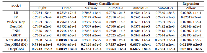
Table 3: Offline performance comparison. AUC (higher is better) is used for binary classification tasks, and MSE (lower is better) is used for regression tasks. All experiments are run 5 times with different random seeds, and the mean ± std results are shown in this table. The top-2 results are marked bold.

표 3: 오프라인 성능 비교. 이진 분류 작업에 AUC(높은 것이 더 좋음)가 사용되고 회귀 작업에 MSE(낮은 것이 더 좋음)가 사용된다. 모든 실험은 다른 랜덤 시드로 5회 실행되며 평균 ± 표준 결과는 이 표에 나와 있습니다. 상위 2개 결과는 굵게 표시됩니다.

Besides, to further analyze the performance of DeepGBM, we use additional two degenerated versions of DeepGBM in experiments:

또한 DeepGBM의 성능을 추가로 분석하기 위해 실험에서 다음과 같은 두 가지 DeepGBM의 퇴화 버전을 추가로 사용합니다.

• DeepGBM (D1), which uses GBDT directly in DeepGBM, rather than GBDT2NN.
  As GBDT cannot be online updated, we can use this model to check the improvement brought by DeepGBM in online scenarios.

  DeepGBM(D1)은 GBDT2NN이 아닌 DeepGBM에서 직접 GBDT를 사용합니다.
  GBDT는 온라인 업데이트가 불가능하므로 이 모델을 사용하여 온라인 시나리오에서 DeepGBM이 개선한 내용을 확인할 수 있습니다.

• DeepGBM (D2), which only uses GBDT2NN in DeepGBM, without CatNN.
  This model is to examine the standalone performance of GBDT2NN.

  DeepGBM(D2)은 CatNN 없이 DeepGBM에서 GBDT2NN만 사용합니다.
  이 모델은 GBDT2NN의 독립 실행형 성능을 검사하기 위한 것이다.

Experiments Settings : To improve the baseline performance, we introduce some basic feature engineering in the experiments.

실험 설정 : 기본 성능을 향상시키기 위해 실험에서 몇 가지 기본 기능 엔지니어링을 소개합니다.

Specifically, for the models which cannot handle numerical features well, such as LR, FM, Wide&Deep, DeepFM and PNN, we discrete the numerical features into categorical ones.

특히 LR, FM, Wide&Deep, DeepFM 및 PNN과 같은 수치 특징을 잘 처리할 수 없는 모델의 경우 수치 특징을 범주형 특징으로 구분한다.

Meanwhile, for the models which cannot handle categorical feature well, such as GBDT and the models based on it, we convert the categorical features into numerical ones, by label-encoding [12] and binary-encoding [41].

한편, GBDT 및 이를 기반으로 하는 모델과 같이 범주형 특징을 잘 처리할 수 없는 모델의 경우 레이블 인코딩 [12] 및 이진 인코딩 [41]을 통해 범주형 특징을 숫자형 특징으로 변환한다.

Based on this basic feature engineering, all models can use the information from both categorical and numerical features, such that the comparisons are more reliable.

이 기본 형상 공학을 기반으로 모든 모델은 범주형 및 수치 형상 모두의 정보를 사용할 수 있으므로 비교가 보다 신뢰할 수 있다.

Moreover, all experiments are run five times with different random seeds to ensure a fair comparison.

또한 공정한 비교를 위해 모든 실험은 서로 다른 무작위 시드로 다섯 번 실행된다.

For the purpose of reproducibility, all the details of experiments settings including hyper-parameter settings will be described in Appendix A and the released codes.

재현성을 위해, 하이퍼 파라미터 설정을 포함한 모든 실험 설정의 세부 사항은 부록 A와 공개된 코드에 설명될 것이다.

4.2 Offline Performance

오프라인 성능

We first evaluate the offline performance for the proposed DeepGBM in this subsection.

먼저 이 하위 절에서 제안된 DeepGBM에 대한 오프라인 성능을 평가한다.

To simulate the real-world scenarios, we partition each benchmark dataset into the training set and test set according to the time-stamp, i.e., the older data samples (about 90%) are used for the training and the newer samples (about 10%) are used for the test. More details are available in Appendix A.

실제 시나리오를 시뮬레이션하기 위해 각 벤치마크 데이터 세트를 시간 스탬프에 따라 훈련 세트와 테스트 세트로 분할한다. 즉, 교육에 오래된 데이터 샘플(약 90%)이 사용되고 테스트에 새로운 샘플(약 10%)이 사용된다. 자세한 내용은 부록 A에서 확인할 수 있습니다.

The overall comparison results could be found in Table 3. From the table, we have following observations:

전체 비교 결과는 표 3에서 확인할 수 있다. 표에 다음과 같은 관찰 결과가 나와 있습니다.

• GBDT can outperform other NN baselines, which explicitly shows the advantage of GBDT on the tabular data. Therefore, distilling GBDT knowledge will definitely benefit DeepGBM.

  GBDT는 다른 NN 기준선을 능가할 수 있으며 표 형식 데이터에서 GBDT의 장점을 명시적으로 보여줍니다. 따라서 GBDT 지식을 습득하면 DeepGBM에 확실히 도움이 될 것입니다.

• GBDT2NN (DeepGBM (D2)) can further improve GBDT, which indicates that GBDT2NN can effectively distill the trained GBDT model into NN. Furthermore, it implies that the distilled NN model can be further improved and even outperform GBDT.

  GBDT2NN(Deep GBM(D2))은 GBDT를 더욱 개선할 수 있으며, 이는 GBDT2NN이 훈련된 GBDT 모델을 NN으로 효과적으로 증류할 수 있음을 나타낸다. 또한 증류된 NN 모델을 더욱 개선하고 GBDT를 능가할 수 있음을 의미한다.

• Combining GBDT and NN can further improve the performance. The hybrid models, including DeepGBM (D1) and DeepGBM, can all reach better performance than single model baselines, which indicates that using two components to handle categorical features and numerical features respectively can benefit performance for online prediction tasks.

  GBDT와 NN을 결합하면 성능을 더욱 향상시킬 수 있습니다. DeepGBM(D1)과 DeepGBM을 포함한 하이브리드 모델은 모두 단일 모델 기준선보다 더 나은 성능에 도달할 수 있으며, 이는 두 구성 요소를 사용하여 각각 범주형 특징과 수치적 특징을 처리하면 온라인 예측 작업의 성능에 도움이 될 수 있음을 나타낸다.

• DeepGBM outperforms all baselines on all datasets. In particular, DeepGBM can boost the accuracy over the best baseline GBDT by 0.3% to 4.4%. as well as the best of NN baselines by 1% to 6.3%.

  DeepGBM은 모든 데이터 세트의 모든 기준선을 능가합니다. 특히 DeepGBM은 최상의 기준 GBDT에 비해 정확도를 0.3%-4.4% 높이고 NN 기준선의 최고치를 1%-6.3% 높일 수 있습니다.

To investigate the convergence of DeepGBM, Fig. 4 demonstrates the performance in terms of AUC on the test data by the model trained with increasing epochs.

DeepGBM의 수렴을 조사하기 위해 그림 4는 증가하는 에포크로 훈련된 모델에 의한 테스트 데이터에 대한 AUC의 성능을 보여준다.

From these figures, we can find that DeepGBM also converges much faster than other models.

이러한 수치를 보면 DeepGBM이 다른 모델보다 훨씬 빠르게 수렴된다는 것을 알 수 있습니다.

4.3 Online Performance

To evaluate the online performance of DeepGBM, we use Flight, Criteo and AutoML-1 datasets as the online benchmark.

DeepGBM의 온라인 성능을 평가하기 위해 Flight, Criteo 및 AutoML-1 데이터 세트를 온라인 벤치마크로 사용한다.

To simulate the online scenarios, we refer to the setting of the “AutoML for Lifelong Machine Learning” Challenge in NeurIPS 2018 [37].

온라인 시나리오를 시뮬레이션하기 위해 뉴런의 "평생 기계 학습을 위한 자동 ML" 과제 설정을 참조한다.IPS 2018 [37].

Specifically, we partition each dataset into multiple consecutive batches along with the time.

특히, 우리는 시간과 함께 각 데이터 세트를 여러 개의 연속적인 배치로 분할한다.

We will train the model for each batch from the oldest to latest in sequence.

우리는 각 배치에 대한 모델을 가장 오래된 것부터 가장 최근의 것 순으로 훈련시킬 것이다.

And, at i-th batch, it only allows to use the samples in that batch to train or update the model; after that, the (i + 1)-th batch is used for the evaluation.

그리고 i-th 배치에서는 해당 배치의 샘플만 사용하여 모델을 훈련하거나 업데이트할 수 있습니다. 그 이후에는 (i + 1)-th 배치가 평가에 사용됩니다.

More details are available in Appendix A.

자세한 내용은 부록 A에서 확인할 수 있습니다.

Note that, as the data distribution may change along with different batches during the online simulation, we would like to examine if the online learned models can perform better than their offline versions, i.e., the models without the online update.

참고로 온라인 시뮬레이션 중에 데이터 배포가 다른 배치와 함께 변경될 수 있으므로 온라인 학습 모델이 오프라인 버전, 즉 온라인 업데이트가 없는 모델보다 더 나은 성능을 발휘할 수 있는지 검사하려고 한다.

Thus, we also check the performance of offline DeepGBM as another baseline to compare with the online learned DeepGBM.

따라서 온라인 학습 DeepGBM과 비교할 수 있는 또 다른 기준으로서 오프라인 DeepGBM의 성능도 점검한다.

All the comparison results are summarized in Fig 5, and we have following observations:

모든 비교 결과는 그림 5에 요약되어 있으며, 다음과 같은 관측 결과가 있습니다.

• GBDT cannot perform well in the online scenarios as expected. Although GBDT yields good result in the first batch (offline stage), it declines obviously in the later (online) batches.

  GBDT는 예상대로 온라인 시나리오에서 제대로 수행할 수 없습니다. GBDT는 첫 번째 배치(오프라인 단계)에서 좋은 결과를 산출하지만, 이후(온라인) 배치에서는 분명히 감소합니다.

• The online performance of GBDT2NN is good. In particular, GBDT2NN (DeepGBM (D2)) can significantly outperform GBDT.

  GBDT2NN의 온라인 성능은 좋습니다. 특히, GBDT2NN(DeepGBM)은 GBDT를 크게 능가할 수 있습니다.

• Furthermore, DeepGBM outperforms DeepGBM (D1), which uses GBDT instead of GBDT2NN, by a non-trivial gain.

  또한 DeepGBM은 GBDT2NN 대신 GBDT를 사용하는 DeepGBM(D1)을 훨씬 능가합니다.

• It indicates that the distilled NN model by GBDT could be further improved and effectively used in the online scenarios.

  이는 GBDT에 의한 증류 NN 모델이 온라인 시나리오에서 더욱 개선되고 효과적으로 사용될 수 있음을 나타낸다.

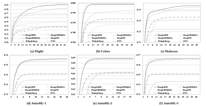
Figure 4: Epoch-AUC curves over test data, in the offline classification experiments.
We can find that DeepGBM converges much faster than other baselines.
Moreover, the convergence points of DeepGBM are also much better.

Figure 4: Epoch-AUC curves over test data, in the offline classification experiments.
We can find that DeepGBM converges much faster than other baselines.
Moreover, the convergence points of DeepGBM are also much better.

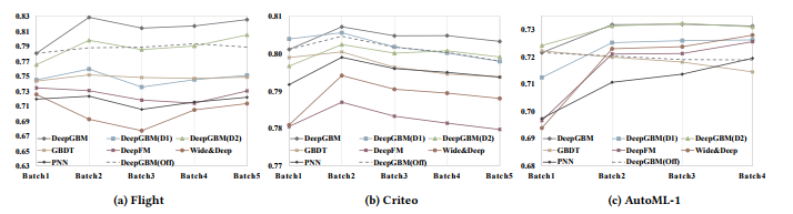
Figure 5: Online performance comparison.
For the models that cannot be online updated, we did not update them during the online simulation.
All experiments are run 5 times with different random seeds, and the mean results (AUC) are used.

그림 5: 온라인 성능 비교.
온라인 업데이트가 불가능한 모델의 경우 온라인 시뮬레이션 중에 업데이트하지 않았습니다.
모든 실험은 서로 다른 랜덤 씨앗을 사용하여 5번 실행되며 평균 결과(AUC)가 사용됩니다.

• DeepGBM outperforms all other baselines, including its offline version (the dotted lines). It explicitly proves the proposed DeepGBM indeed yields strong learning capacity over both categorical and numerical tabular features while retaining the vital ability of efficient online learning.

  DeepGBM은 오프라인 버전(점선)을 포함하여 다른 모든 기준선을 능가합니다. 이는 제안된 DeepGBM이 효율적인 온라인 학습의 필수적인 능력을 유지하면서 범주형 및 수치형 특징 모두에 대해 강력한 학습 능력을 제공한다는 것을 분명히 입증한다.

In short, all above experimental results demonstrate that DeepGBM can significantly outperform all kinds of baselines in both offline and online scenarios.

간단히 말해서 위의 모든 실험 결과는 DeepGBM이 오프라인 및 온라인 시나리오 모두에서 모든 종류의 기준선을 크게 능가할 수 있음을 보여준다.

5. CONCLUSION

결론

To address the challenges of tabular input space, which indicates the existence of both sparse categorical features and dense numerical ones, and online data generation, which implies continuous taskgenerated data with potentially dynamic distribution, in online prediction tasks, we propose a new learning framework, DeepGBM, which integrates NN and GBDT together.

온라인 예측 작업에서 희박한 범주형 특징과 밀도가 높은 수치적 특징의 존재를 나타내는 표 입력 공간과 잠재적으로 동적 분포가 있는 지속적인 작업 생성 데이터를 의미하는 온라인 데이터 생성의 과제를 해결하기 위해 NN A를 통합하는 새로운 학습 프레임워크인 DeepGBM을 제안한다.GBDT를 함께 사용합니다.

Specifically, DeepGBM consists of two major components: CatNN being an NN structure with the input of sparse categorical features and GBDT2NN being another NN structure with the input of dense numerical features.

특히 DeepGBM은 두 가지 주요 구성 요소로 구성된다. CatNN은 희소 범주 형상의 입력이 있는 NN 구조이고 GBDT2NN은 밀도가 높은 수치 형상의 입력이 있는 또 다른 NN 구조이다.

To further take advantage of GBDT’s strength in learning over dense numerical features, GBDT2NN attempts to distill the knowledge learned by GBDT into an NN modeling process.

GBDT2NN은 고밀도 수치 특징을 학습하는 GBDT의 강점을 더욱 활용하기 위해 GBDT에서 학습한 지식을 NN 모델링 프로세스로 증류하려고 한다.

Powered by these two NN based components, DeepGBM can indeed yield the strong learning capacity over both categorical and numerical tabular features while retaining the vital ability of efficient online learning.

이 두 NN 기반 구성 요소에 의해 구동되는 DeepGBM은 효율적인 온라인 학습의 중요한 능력을 유지하면서 범주형 및 수치형 특징 모두에 대해 강력한 학습 용량을 제공할 수 있다.

Comprehensive experimental results demonstrate that DeepGBM can outperform other solutions in various prediction tasks, in both offline and online scenarios.

종합적인 실험 결과는 DeepGBM이 오프라인 및 온라인 시나리오 모두에서 다양한 예측 작업에서 다른 솔루션을 능가할 수 있음을 보여준다.

REFERENCES

[1] Eugene Agichtein, Eric Brill, and Susan Dumais. 2006. Improving web search ranking by incorporating user behavior information. In Proceedings of the 29th annual international ACM SIGIR conference on Research and development in information retrieval. ACM, 19–26.

[2] Arunava Banerjee. 1997. Initializing neural networks using decision trees. Computational learning theory and natural learning systems 4 (1997), 3–15.

[3] Iñigo Barandiaran. 1998. The random subspace method for constructing decision
forests. IEEE transactions on pattern analysis and machine intelligence 20, 8 (1998). [4] Yael Ben-Haim and Elad Tom-Tov. 2010. A streaming parallel decision tree algorithm. Journal of Machine Learning Research 11, Feb (2010), 849–872.

[5] Gérard Biau, Erwan Scornet, and Johannes Welbl. 2016. Neural random forests. Sankhya A (2016), 1–40.
[6] Christopher JC Burges. 2010. From ranknet to lambdarank to lambdamart: An overview. Learning 11, 23-581 (2010), 81.

[7] Zhe Cao, Tao Qin, Tie-Yan Liu, Ming-Feng Tsai, and Hang Li. 2007. Learning to rank: from pairwise approach to listwise approach. In Proceedings of the 24th international conference on Machine learning. ACM, 129–136.

[8] Tianqi Chen and Carlos Guestrin. 2016. Xgboost: A scalable tree boosting system. In Proceedings of the 22nd acm sigkdd international conference on knowledge discovery and data mining. ACM, 785–794.

[9] Heng-Tze Cheng, Levent Koc, Jeremiah Harmsen, Tal Shaked, Tushar Chandra, Hrishi Aradhye, Glen Anderson, Greg Corrado, Wei Chai, Mustafa Ispir, et al. 2016. Wide & deep learning for recommender systems. In Proceedings of the 1st Workshop on Deep Learning for Recommender Systems. ACM, 7–10.

[10] Paul Covington, Jay Adams, and Emre Sargin. 2016. Deep neural networks for youtube recommendations. In Proceedings of the 10th ACM Conference on Recommender Systems. ACM, 191–198.

[11] Pedro Domingos and Geoff Hulten. 2000. Mining high-speed data streams. In Proceedings of the sixth ACM SIGKDD international conference on Knowledge discovery and data mining. ACM, 71–80.

[12] Anna Veronika Dorogush, Vasily Ershov, and Andrey Gulin. 2018. CatBoost: gradient boosting with categorical features support. arXiv preprint arXiv:1810.11363 (2018).

[13] James Dougherty, Ron Kohavi, and Mehran Sahami. 1995. Supervised and unsupervised discretization of continuous features. In Machine Learning Proceedings 1995. Elsevier, 194–202.

[14] Ji Feng, Yang Yu, and Zhi-Hua Zhou. 2018. Multi-Layered Gradient Boosting Decision Trees. arXiv preprint arXiv:1806.00007 (2018).

[15] Manuel Fernández-Delgado, Eva Cernadas, Senén Barro, and Dinani Amorim. Do we need hundreds of classifiers to solve real world classification problems? The Journal of Machine Learning Research 15, 1 (2014), 3133–3181.

[16] Jerome Friedman, Trevor Hastie, and Robert Tibshirani. 2001. The elements of statistical learning. Vol. 1. Springer series in statistics New York, NY, USA:.

[17] Jerome H Friedman. 2001. Greedy function approximation: a gradient boosting machine. Annals of statistics (2001), 1189–1232.

[18] Mohamed Medhat Gaber, Arkady Zaslavsky, and Shonali Krishnaswamy. 2005. Mining data streams: a review. ACM Sigmod Record 34, 2 (2005), 18–26.

[19] Ian Goodfellow, Yoshua Bengio, Aaron Courville, and Yoshua Bengio. 2016. Deep learning. Vol. 1. MIT press Cambridge.

[20] Krzysztof Grabczewski and Norbert Jankowski. 2005. Feature selection with decision tree criterion. In null. IEEE, 212–217.

[21] Thore Graepel, Joaquin Quinonero Candela, Thomas Borchert, and Ralf Herbrich. 2010. Web-scale bayesian click-through rate prediction for sponsored search advertising in microsoft’s bing search engine. Omnipress.

[22] Huifeng Guo, Ruiming Tang, Yunming Ye, Zhenguo Li, and Xiuqiang He. 2017. Deepfm: a factorization-machine based neural network for ctr prediction. arXiv preprint arXiv:1703.04247 (2017).

[23] Xinran He, Junfeng Pan, Ou Jin, Tianbing Xu, Bo Liu, Tao Xu, Yanxin Shi, Antoine Atallah, Ralf Herbrich, Stuart Bowers, et al. 2014. Practical lessons from predicting clicks on ads at facebook. In Proceedings of the Eighth International Workshop on Data Mining for Online Advertising. ACM, 1–9.

[24] Geoffrey Hinton, Oriol Vinyals, and Jeff Dean. 2015. Distilling the knowledge in a neural network. arXiv preprint arXiv:1503.02531 (2015).

[25] K. D. Humbird, J. L. Peterson, and R. G. McClarren. 2017. Deep neural network initialization with decision trees. ArXiv e-prints (July 2017). arXiv:1707.00784

[26] Yani Ioannou, Duncan Robertson, Darko Zikic, Peter Kontschieder, Jamie Shotton, Matthew Brown, and Antonio Criminisi. 2016. Decision forests, convolutional networks and the models in-between. arXiv preprint arXiv:1603.01250 (2016).

[27] Sergey Ioffe and Christian Szegedy. 2015. Batch normalization: Accelerating deep network training by reducing internal covariate shift. arXiv preprint arXiv:1502.03167 (2015).

[28] Ruoming Jin and Gagan Agrawal. 2003. Efficient decision tree construction on streaming data. In Proceedings of the ninth ACM SIGKDD international conference on Knowledge discovery and data mining. ACM, 571–576.

[29] Guolin Ke, Qi Meng, Thomas Finley, Taifeng Wang, Wei Chen, Weidong Ma, Qiwei Ye, and Tie-Yan Liu. 2017. LightGBM: A highly efficient gradient boosting decision tree. In Advances in Neural Information Processing Systems. 3146–3154.

[30] Peter Kontschieder, Madalina Fiterau, Antonio Criminisi, and Samuel Rota Bulo. 2015 Deep neural decision forests. In Proceedings of the IEEE international conference on computer vision. 1467–1475.

[31] Yaguang Li, Kun Fu, Zheng Wang, Cyrus Shahabi, Jieping Ye, and Yan Liu. 2018. Multi-task representation learning for travel time estimation. In International Conference on Knowledge Discovery and Data Mining,(KDD).

[32] Jianxun Lian, Xiaohuan Zhou, Fuzheng Zhang, Zhongxia Chen, Xing Xie, and Guangzhong Sun. 2018. xDeepFM: Combining Explicit and Implicit Feature Interactions for Recommender Systems. arXiv preprint arXiv:1803.05170 (2018).

[33] Xiaoliang Ling, Weiwei Deng, Chen Gu, Hucheng Zhou, Cui Li, and Feng Sun. Model ensemble for click prediction in bing search ads. In Proceedings of the 26th International Conference on World Wide Web Companion. International World Wide Web Conferences Steering Committee, 689–698.

[34] Qi Meng, Guolin Ke, Taifeng Wang, Wei Chen, Qiwei Ye, Zhi-Ming Ma, and Tie-Yan Liu. 2016. A communication-efficient parallel algorithm for decision tree. In Advances in Neural Information Processing Systems. 1279–1287.

[35] Tomas Mikolov, Kai Chen, Greg Corrado, and Jeffrey Dean. 2013. Efficient estimation of word representations in vector space. arXiv preprint arXiv:1301.3781
(2013).

[36] Yanru Qu, Han Cai, Kan Ren, Weinan Zhang, Yong Yu, Ying Wen, and Jun Wang. 2016. Product-based neural networks for user response prediction. In Data Mining (ICDM), 2016 IEEE 16th International Conference on. IEEE, 1149–1154.

[37] Yao Quanming, Wang Mengshuo, Jair Escalante Hugo, Guyon Isabelle, Hu Yi-Qi, Li Yu-Feng, Tu Wei-Wei, Yang Qiang, and Yu Yang. 2018. Taking human out of learning applications: A survey on automated machine learning. arXiv preprint arXiv:1810.13306 (2018).

[38] Steffen Rendle. 2010. Factorization machines. In Data Mining (ICDM), 2010 IEEE 10th International Conference on. IEEE, 995–1000.

[39] David L Richmond, Dagmar Kainmueller, Michael Y Yang, Eugene W Myers, and Carsten Rother. 2015. Relating cascaded random forests to deep convolutional neural networks for semantic segmentation. arXiv preprint arXiv:1507.07583 (2015).

[40] Samuel Rota Bulo and Peter Kontschieder. 2014. Neural decision forests for semantic image labelling. In Proceedings of the IEEE Conference on Computer Vision and Pattern Recognition. 81–88.

[41] Scikit-learn. 2018. categorical_encoding. https://github.com/scikitlearncontrib/ categoricalencoding.

[42] Ishwar Krishnan Sethi. 1990. Entropy nets: from decision trees to neural networks. Proc. IEEE 78, 10 (1990), 1605–1613.

[43] Ira Shavitt and Eran Segal. 2018. Regularization Learning Networks: Deep Learning for Tabular Datasets. In Advances in Neural Information Processing Systems. 1386–1396.

[44] Jeany Son, Ilchae Jung, Kayoung Park, and Bohyung Han. 2015. Tracking-bysegmentation with online gradient boosting decision tree. In Proceedings of the IEEE International Conference on Computer Vision. 3056–3064.

[45] V Sugumaran, V Muralidharan, and KI Ramachandran. 2007. Feature selection using decision tree and classification through proximal support vector machine for fault diagnostics of roller bearing. Mechanical systems and signal processing 21, 2 (2007), 930–942.

[46] Christian Szegedy, Wei Liu, Yangqing Jia, Pierre Sermanet, Scott Reed, Dragomir Anguelov, Dumitru Erhan, Vincent Vanhoucke, and Andrew Rabinovich. 2015. Going deeper with convolutions. In Proceedings of the IEEE conference on computer vision and pattern recognition. 1–9.

[47] Hao Wang, Naiyan Wang, and Dit-Yan Yeung. 2015. Collaborative deep learning for recommender systems. In Proceedings of the 21th ACM SIGKDD International Conference on Knowledge Discovery and Data Mining. ACM, 1235–1244.

[48] Suhang Wang, Charu Aggarwal, and Huan Liu. 2017. Using a random forest to inspire a neural network and improving on it. In Proceedings of the 2017 SIAM International Conference on Data Mining. SIAM, 1–9.

[49] Zheng Wang, Kun Fu, and Jieping Ye. 2018. Learning to estimate the travel time. In Proceedings of the 24th ACM SIGKDD International Conference on Knowledge Discovery & Data Mining. ACM, 858–866.

[50] Yongxin Yang, Irene Garcia Morillo, and Timothy M Hospedales. 2018. Deep Neural Decision Trees. arXiv preprint arXiv:1806.06988 (2018).

[51] Weinan Zhang, Tianming Du, and Jun Wang. 2016. Deep learning over multi-field
categorical data. In European conference on information retrieval. Springer, 45–57. [52] Zhi-Hua Zhou and Ji Feng. 2017. Deep forest: Towards an alternative to deep
neural networks. arXiv preprint arXiv:1702.08835 (2017).

[53] Jie Zhu, Ying Shan, JC Mao, Dong Yu, Holakou Rahmanian, and Yi Zhang. 2017. Deep embedding forest: Forest-based serving with deep embedding features. In Proceedings of the 23rd ACM SIGKDD International Conference on Knowledge Discovery and Data Mining. ACM, 1703–1711.