• 주제 : Generative Adversarial Networks
• 논문 : Generative Adversarial Networks
• 논문 링크 : https://arxiv.org/abs/1406.2661

Abstract

We propose a new framework for estimating generative models via an adversarial process, in which we simultaneously train two models: a generative model G that captures the data distribution, and a discriminative model D that estimates the probability that a sample came from the training data rather than G.

The training procedure for G is to maximize the probability of D making a mistake.

This framework corresponds to a minimax two-player game. In the space of arbitrary functions G and D, a unique solution exists, with G recovering the training data distribution and D equal to 21 everywhere.

In the case where G and D are defined by multilayer perceptrons, the entire system can be trained with backpropagation.

There is no need for any Markov chains or unrolled approximate inference net- works during either training or generation of samples.

Experiments demonstrate the potential of the framework through qualitative and quantitative evaluation of the generated samples.

1. Introdution

The promise of deep learning is to discover rich, hierarchical models that represent probability distributions over the kinds of data encountered in artificial intelligence applications, such as natural images, audio waveforms containing speech, and symbols in natural language corpora.

So far, the most striking successes in deep learning have involved discriminative models, usually those that map a high-dimensional, rich sensory input to a class label.

These striking successes have primarily been based on the backpropagation and dropout algorithms, using piecewise linear units which have a particularly well-behaved gradient .

Deep generative models have had less of an impact, due to the difficulty of approximating many intractable probabilistic computations that arise in maximum likelihood estimation and related strategies, and due to difficulty of leveraging the benefits of piecewise linear units in the generative context.

We propose a new generative model estimation procedure that sidesteps these difficulties.

In the proposed adversarial nets framework, the generative model is pitted against an adversary: a discriminative model that learns to determine whether a sample is from the model distribution or the data distribution.

The generative model can be thought of as analogous to a team of counterfeiters, trying to produce fake currency and use it without detection, while the discriminative model is analogous to the police, trying to detect the counterfeit currency.

Competition in this game drives both teams to improve their methods until the counterfeits are indistiguishable from the genuine articles.

This framework can yield specific training algorithms for many kinds of model and optimization algorithm.

In this article, we explore the special case when the generative model generates samples by passing random noise through a multilayer perceptron, and the discriminative model is also a multilayer perceptron.

We refer to this special case as adversarial nets.

In this case, we can train both models using only the highly successful backpropagation and dropout algorithms and sample from the generative model using only forward propagation.

No approximate inference or Markov chains are necessary.

2. Related Work

An alternative to directed graphical models with latent variables are undirected graphical models with latent variables, such as restricted Boltzmann machines (RBMs), deep Boltzmann machines (DBMs) and their numerous variants.

The interactions within such models are represented as the product of unnormalized potential functions, normalized by a global summation/integration over all states of the random variables.

This quantity (the partition function) and its gradient are intractable for all but the most trivial instances, although they can be estimated by Markov chain Monte Carlo (MCMC) methods.

Mixing poses a significant problem for learning algorithms that rely on MCMC.

Deep belief networks (DBNs) are hybrid models containing a single undirected layer and sev- eral directed layers.

While a fast approximate layer-wise training criterion exists, DBNs incur the computational difficulties associated with both undirected and directed models.

Alternative criteria that do not approximate or bound the log-likelihood have also been proposed, such as score matching and noise-contrastive estimation (NCE).

Both of these require the learned probability density to be analytically specified up to a normalization constant.

Note that in many interesting generative models with several layers of latent variables (such as DBNs and DBMs), it is not even possible to derive a tractable unnormalized probability density.

Some models such as denoising auto-encoders and contractive autoencoders have learning rules very similar to score matching applied to RBMs.

In NCE, as in this work, a discriminative training criterion is employed to fit a generative model.

However, rather than fitting a separate discriminative model, the generative model itself is used to discriminate generated data from samples a fixed noise distribution.

Because NCE uses a fixed noise distribution, learning slows dramatically after the model has learned even an approximately correct distribution over a small subset of the observed variables.

Finally, some techniques do not involve defining a probability distribution explicitly, but rather train a generative machine to draw samples from the desired distribution.

This approach has the advantage that such machines can be designed to be trained by back-propagation.

Prominent recent work in this area includes the generative stochastic network (GSN) framework, which extends generalized denoising auto-encoders: both can be seen as defining a parameterized Markov chain, i.e., one learns the parameters of a machine that performs one step of a generative Markov chain.

Compared to GSNs, the adversarial nets framework does not require a Markov chain for sampling.

Because adversarial nets do not require feedback loops during generation, they are better able to leverage piecewise linear units, which improve the performance of backpropagation but have problems with unbounded activation when used ina feedback loop.

More recent examples of training a generative machine by back-propagating into it include recent work on auto-encoding variational Bayes and stochastic backpropagation.

3. Adversarial nets

The adversarial modeling framework is most straightforward to apply when the models are both multilayer perceptrons.

To learn the generator’s distribution $p_g$ over data $x$, we define a prior on input noise variables $p_z(z)$, then represent a mapping to data space as $G(z;θ_g)$, where $G$ is a differentiable function represented by a multilayer perceptron with parameters $θ_g$.

We also define a second multilayer perceptron $D(x; θ_d)$ that outputs a single scalar.
$D(x)$ represents the probability that $x$ came from the data rather than $p_g$.

We train $D$ to maximize the probability of assigning the correct label to both training examples and samples from $G$.

We simultaneously train $G$ to minimize $log(1 − D(G(z)))$:
In other words, $D$ and $G$ play the following two-player minimax game with value function $V(G, D)$:

In the next section, we present a theoretical analysis of adversarial nets, essentially showing that the training criterion allows one to recover the data generating distribution as $G$ and $D$ are given enough capacity, i.e., in the non-parametric limit.

See Figure 1 for a less formal, more pedagogical explanation of the approach.

In practice, we must implement the game using an iterative, numerical approach.

Optimizing $D$ to completion in the inner loop of training is computationally prohibitive, and on finite datasets would result in overfitting.

Instead, we alternate between $k$ steps of optimizing $D$ and one step of optimizing $G$.

This results in $D$ being maintained near its optimal solution, so long as $G$ changes slowly enough.

This strategy is analogous to the way that SML/PCD training maintains samples from a Markov chain from one learning step to the next in order to avoid burning in a Markov chain as part of the inner loop of learning.

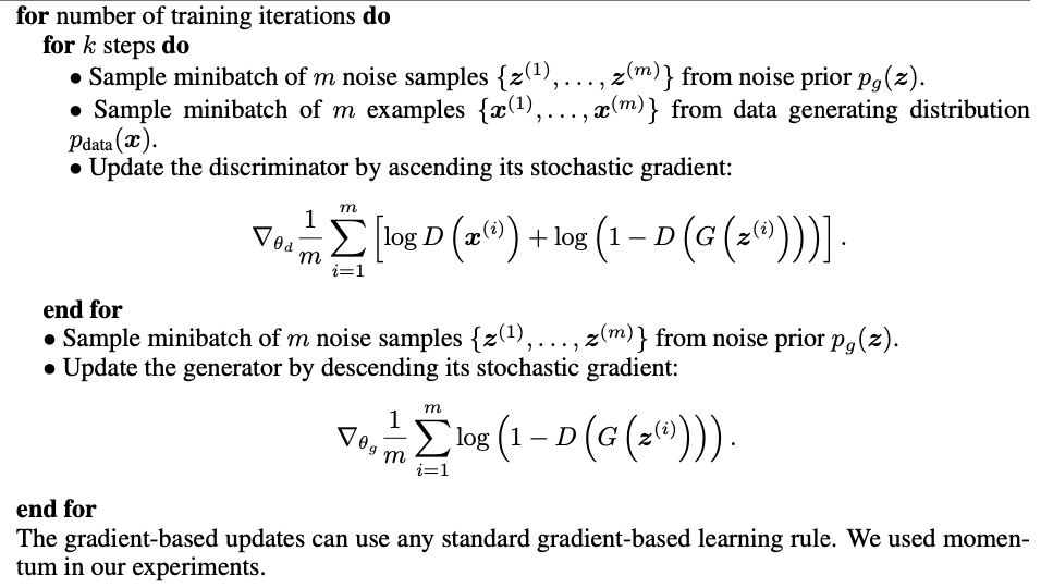
The procedure is formally presented in Algorithm 1.

In practice, equation 1 may not provide sufficient gradient for $G$ to learn well.

Early in learning, when $G$ is poor, $D$ can reject samples with high confidence because they are clearly different from the training data.

In this case, $log(1 − D(G(z)))$ saturates.

Rather than training $G$ to minimize $log(1 − D(G(z)))$ we can train $G$ to maximize $log D(G(z))$.

This objective function results in the same fixed point of the dynamics of $G$ and $D$ but provides much stronger gradients early in learning.

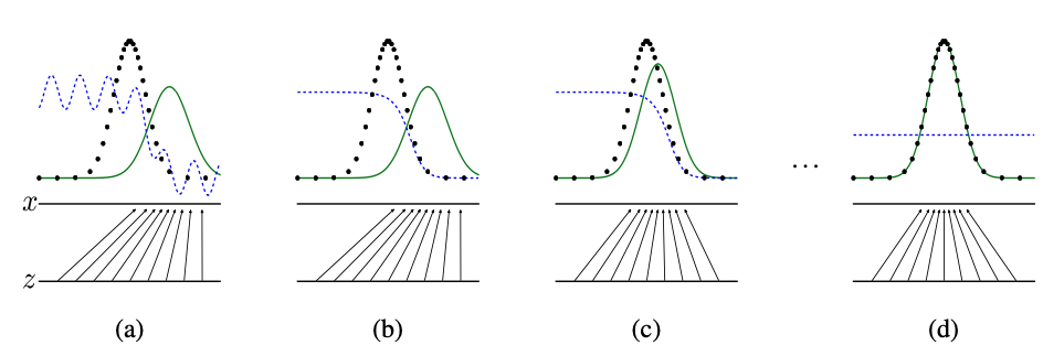
Figure 1: Generative adversarial nets are trained by simultaneously updating the discriminative distribution (D, blue, dashed line) so that it discriminates between samples from the data generating distribution (black, dotted line) px from those of the generative distribution $p_g$ (G) (green, solid line).

The lower horizontal line is the domain from which $z$ is sampled, in this case uniformly.

The horizontal line above is part of the domain of $x$.

The upward arrows show how the mapping $x = G(z)$ imposes the non-uniform distribution pg on transformed samples.

$G$ contracts in regions of high density and expands in regions of low density of $P_g$.

(a) Consider an adversarial pair near convergence: $P_g$ is similar to pdata and $D$ is a partially accurate classifier.

(b) In the inner loop of the algorithm $D$ is trained to discriminate samples from data, converging to $D^∗(x) = \frac{P_{data}(x)}{P_{data}(x)+P_g(x)}$ .

(c) After an update to $G$, gradient of D has guided $G(z)$ to flow to regions that are more likely to be classified as data.

(d) After several steps of training, if $G$ and $D$ have enough capacity, they will reach a point at which both cannot improve because $P_g = P_{data}$.
The discriminator is unable to differentiate between the two distributions, i.e. $D(x) = \frac{1}{2}$.

4. Theoretical Results

The generator $G$ implicitly defines a probability distribution pg as the distribution of the samples $G(z)$ obtained when $z ∼ pz$.

Therefore, we would like Algorithm 1 to converge to a good estimator of $p_{data}$, if given enough capacity and training time.

The results of this section are done in a non- parametric setting, e.g. we represent a model with infinite capacity by studying convergence in the space of probability density functions.

We will show in section 4.1 that this minimax game has a global optimum for $p_g = p_{data}$.

We will then show in section 4.2 that Algorithm 1 optimizes Eq 1, thus obtaining the desired result.

Algorithm 1

Minibatch stochastic gradient descent training of generative adversarial nets.
The number of steps to apply to the discriminator, $k$, is a hyperparameter.
We used $k = 1$, the least expensive option, in our experiments.

4.1 Global Optimality of ${P_g=P_{data}}$

We first consider the optimal discriminator $D$ for any given generator $G$.

Proposition 1. For $G$ fixed, the optimal discriminator $D$ is

Proof. The training criterion for the discriminator $D$, given any generator $G$, is to maximize the quantity $V (G, D)$

For any $(a, b) ∈ R^2 / {0, 0}$, the function $y → alog(y) + blog(1 − y)$ achieves its maximum in [0,1] at $\frac{a}{a+b}$.
The discriminator does not need to be defined outside of $Supp(P_{data}) ∪ Supp(P_g)$, concluding the proof.

Note that the training objective for $D$ can be interpreted as maximizing the log-likelihood for estimating the conditional probability $P(Y = y|x)$, where $Y$ indicates whether $x$ comes from $P_{data}$(with y = 1) or from $p_g$(with y = 0).
The minimax game in Eq. 1 can now be reformulated as:

Theorem 1. The global minimum of the virtual training criterion $C(G)$ is achieved if and only if $P_g =P_{data}$.
Atthatpoint, $C(G)$ achieves the value − log4.

Proof. For $P_g = P_{data}$ , $D_G^∗(x) = \frac{1}{2}$, (consider Eq. 2).
Hence, by inspecting Eq. 4 at $D_G^∗ (x) = \frac{1}{2}$,
we find $C(G) = log \frac{1}{2} + log \frac{1}{2} = − log 4.$
To see that this is the best possible value of $C(G)$,
reached only for $P_g = P_{data}$, observe that

and that by subtracting this expression from $C(G) = V (D_G^∗, G)$, we obtain:

where KL is the Kullback–Leibler divergence.
We recognize in the previous expression the Jensen–Shannon divergence between the model’s distribution and the data generating process:

Since the Jensen–Shannon divergence between two distributions is always non-negative and zero only when they are equal, we have shown that $C^∗ = − log(4)$ is the global minimum of $C(G)$ and that the only solution is $P_g=P_{data}$,i.e., the generative model perfectly replicating the data generating process.

4.2 Convergence of Algorithm 1

Proposition 2. If G and D have enough capacity, and at each step of Algorithm 1, the discriminator is allowed to reach its optimum given G, and pg is updated so as to improve the criterion

hen $P_g$ converges to $P_{data}$

Proof. Consider $V(G,D) = U(P_g,D)$ as a function of pg as done in the above criterion. Note that $U(P_g,D)$ is convex in $P_g$.

The subderivatives of a supremum of convex functions include the derivative of the function at the point where the maximum is attained.

In other words, if $f(x) = sup_{α∈A}f_α(x)$ and $f_α(x)$ is convex in $x$ for every $α$, then $∂fβ(x) ∈ ∂f$ if $β = argsup_{α∈A}f_α(x)$.

This is equivalent to computing a gradient descent update for pg at the optimal $D$ given the corresponding $G$.

supD U(pg,D) is convex in $P_g$ with a unique global optima as proven in Thm 1, therefore with sufficiently small updates of $P_g, P_g$ converges to $P_x$, concluding the proof.

In practice, adversarial nets represent a limited family of $P_g$ distributions via the function $G(z; θ_g )$, and we optimize $θ_g$ rather than pg itself.

Using a multilayer perceptron to define $G$ introduces multiple critical points in parameter space.

However, the excellent performance of multilayer perceptrons in practice suggests that they are a reasonable model to use despite their lack of theoretical guarantees.

5. Experiments

We trained adversarial nets an a range of datasets including MNIST, the Toronto Face Database (TFD), and CIFAR-10.
The generator nets used a mixture of rectifier linear activations and sigmoid activations, while the discriminator net used maxout activations.
Dropout was applied in training the discriminator net.
While our theoretical framework permits the use of dropout and other noise at intermediate layers of the generator, we used noise as the input to only the bottommost layer of the generator network.

We estimate probability of the test set data under $P_g$ by fitting a Gaussian Parzen window to the samples generated with $G$ and reporting the log-likelihood under this distribution.

model	MNIST	TFD
DBN	138 $\pm$ 2	1909 $\pm$ 66
Stacked CAE	121 $\pm$ 1.6	2110 $\pm$ 50
Deep GSN	214 $\pm$ 1.1	1890 $\pm$ 29
Adversarial	225 $\pm$ 2	2057 $\pm$ 26

Table 1: Parzen window-based log-likelihood estimates.
The reported numbers on MNIST are the mean log- likelihood of samples on test set, with the standard error of the mean computed across examples.
On TFD, we computed the standard error across folds of the dataset, with a different σ chosen using the validation set of each fold.
On TFD, $σ$ was cross validated on each fold and mean log-likelihood on each fold were computed.
For MNIST we compare against other models of the real-valued (rather than binary) version of dataset.

The $σ$ parameter of the Gaussians was obtained by cross validation on the validation set.
This procedure was introduced in Breuleux et al. and used for various generative models for which the exact likelihood is not tractable.
Results are reported in Table 1.
This method of estimating the likelihood has somewhat high variance and does not perform well in high dimensional spaces but it is the best method available to our knowledge.
Advances in generative models that can sample but not estimate likelihood directly motivate further research into how to evaluate such models.

In Figures 2 and 3 we show samples drawn from the generator net after training.
While we make no claim that these samples are better than samples generated by existing methods, we believe that these samples are at least competitive with the better generative models in the literature and highlight the potential of the adversarial framework.

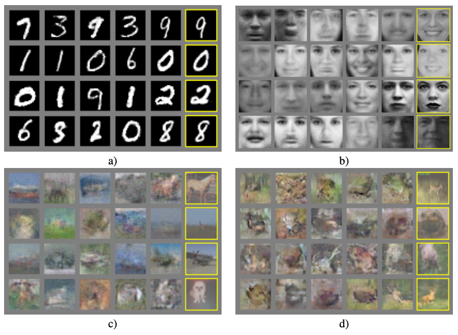
Figure 2: Visualization of samples from the model. Rightmost column shows the nearest training example of the neighboring sample, in order to demonstrate that the model has not memorized the training set.
Samples are fair random draws, not cherry-picked.
Unlike most other visualizations of deep generative models, these images show actual samples from the model distributions, not conditional means given samples of hidden units.
Moreover, these samples are uncorrelated because the sampling process does not depend on Markov chain mixing.
a) MNIST b) TFD c) CIFAR-10 (fully connected model) d) CIFAR-10 (convolutional discriminator and “deconvolutional” generator)

Figure 3: Digits obtained by linearly interpolating between coordinates in $z$ space of the full model.

	Deep directed graphical models	Deep undirected graphical models	Generative autoencoders	Adversarial models
Training	Inference needed during training.	Inference needed during training. MCMC needed to approximate partition function gradient.	Enforced tradeoff between mixing and power of reconstruction generation	Synchronizing the discriminator with the generator. Helvetica.
Inference	27	Variational inference	MCMC-based inference	Learned approximate inference
Sampling	No difficulties	Requires Markov chain	Requires Markov chain	No difficulties
Evaluating $p(x)$	Intractable, may be approximated with AIS	Intractable, may be approximated with AIS	Not explicitly represented, may be approximated with Parzen density estimation	Not explicitly represented, may be approximated with Parzen density estimation
Model design	Nearly all models incur extreme difficulty	Careful design needed to ensure multiple properties	Any differentiable function is theoretically permitted	Any differentiable function is theoretically permitted

Table 2: Challenges in generative modeling: a summary of the difficulties encountered by different approaches to deep generative modeling for each of the major operations involving a model.

6. Advantages and disadvantages

This new framework comes with advantages and disadvantages relative to previous modeling frameworks.
The disadvantages are primarily that there is no explicit representation of $P_g(x)$, and that $D$ must be synchronized well with $G$ during training (in particular, $G$ must not be trained too much without updating $D$, in order to avoid “the Helvetica scenario” in which $G$ collapses too many values of $z$ to the same value of $x$ to have enough diversity to model pdata), much as the negative chains of a Boltzmann machine must be kept up to date between learning steps.
The advantages are that Markov chains are never needed, only backprop is used to obtain gradients, no inference is needed during learning, and a wide variety of functions can be incorporated into the model.
Table 2 summarizes the comparison of generative adversarial nets with other generative modeling approaches.

The aforementioned advantages are primarily computational.
Adversarial models may also gain some statistical advantage from the generator network not being updated directly with data examples, but only with gradients flowing through the discriminator.
This means that components of the input are not copied directly into the generator’s parameters.
Another advantage of adversarial networks is that they can represent very sharp, even degenerate distributions, while methods based on Markov chains require that the distribution be somewhat blurry in order for the chains to be able to mix between modes.

7. Conlusions and future work

This framework admits many straightforward extensions:

1. A $conditional generative$ model $P(x | c)$ can be obtained by adding $c$ as input to both $G$ and $D$.
2. $Learned approximate inference$ can be performed by training an auxiliary network to predict $z$ given $x$.
   This is similar to the inference net trained by the wake-sleep algorithm but with the advantage that the inference net may be trained for a fixed generator net after the generator net has finished training.
3. One can approximately model all conditionals $P(x_S | x_S)$ where $S$ is a subset of the indices of $x$ by training a family of conditional models that share parameters.
   Essentially, one can use adversarial nets to implement a stochastic extension of the deterministic MP-DBM.
4. Semi-supervised learning: features from the discriminator or inference net could improve perfor- mance of classifiers when limited labeled data is available.
5. Efficiency improvements: training could be accelerated greatly by divising better methods for coordinating $G$ and $D$ or determining better distributions to sample $z$ from during training.