Summary

Newton's Method

This sets the stage for Newton's method, which starts with an initial approximation $p_0$ and generates the sequence $\left\{p_n\right\}_{n=0}^{\infty}$, by

이것은 초기 근사 $p_0$로 시작하여 $\left\{p_n\right\}_{n=0}^{\infty}$ 시퀀스를 생성하는 뉴턴의 방법의 단계를 설정한다.

Convergence Theorem for Newton's Method

• Let $f \in C^2[a, b]$. If $p \in(a, b)$ is such that $f(p)=0$ and $f^{\prime}(p) \neq 0$.
• Then there exists a $\delta>0$ such that Newton's method generates a sequence $\left\{p_n\right\}_{n=1}^{\infty}$, defined by

$f \in C^2[a, b]$로 하자. $p \in(a, b)$가 $f(p)=0$ 및 $f^{\prime}(p) \neq 0$과 같은 경우.
그런 다음 뉴턴의 방법이 다음과 같이 정의된 $\left\{p_n\right\}_{n=1}^{\infty}$ 시퀀스를 생성하도록 $\delta>0$ 이 존재한다.

converging to $p$ for any initial approximation

초기 근사치에 대해 $p$로 수렴

The Secant Method

Newton's Method: Derivation

Newton's Method

Context

Newton's (or the Newton-Raphson) method is one of the most powerful and well-known numerical methods for solving a root-finding problem.

뉴턴의 방법(또는 뉴턴-랩슨)은 근을 찾는 문제를 해결하기 위한 가장 강력하고 잘 알려진 수치적 방법 중 하나이다.

Various ways of introducing Newton's method

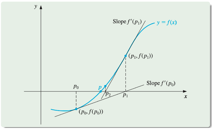
• Graphically, as is often done in calculus.
• As a technique to obtain faster convergence than offered by other types of functional iteration.
• Using Taylor polynomials. We will see there that this particular derivation produces not only the method, but also a bound for the error of the approximation.

그래픽적으로는 미적분학에서 흔히 행해지는 것과 같다.
다른 유형의 기능 반복에 의해 제공되는 것보다 더 빠른 수렴을 얻기 위한 기술입니다.
테일러 다항식 사용. 우리는 여기서 이 특정 파생이 방법뿐만 아니라 근사 오차에 대한 경계를 생성한다는 것을 알게 될 것이다.

Derivation

• Suppose that $f \in C^2[a, b]$. Let $p_0 \in[a, b]$ be an approximation to $p$ such that $f^{\prime}\left(p_0\right) \neq 0$ and $\left|p-p_0\right|$ is "small."
• Consider the first Taylor polynomial for $f(x)$ expanded about $p_0$ and evaluated at $x=p$.
  $f(p)=f\left(p_0\right)+\left(p-p_0\right) f^{\prime}\left(p_0\right)+\frac{\left(p-p_0\right)^2}{2} f^{\prime \prime}(\xi(p)),$
  where $\xi(p)$ lies between $p$ and $p_0$.
• Since $f(p)=0$, this equation gives
  $0=f\left(p_0\right)+\left(p-p_0\right) f^{\prime}\left(p_0\right)+\frac{\left(p-p_0\right)^2}{2} f^{\prime \prime}(\xi(p)) .$

Derivation (Cont'd)

• Newton's method is derived by assuming that since $\left|p-p_0\right|$ is small, the term involving $\left(p-p_0\right)^2$ is much smaller, so
  $0 \approx f\left(p_0\right)+\left(p-p_0\right) f^{\prime}\left(p_0\right) .$
• Solving for $p$ gives
  $p \approx p_0-\frac{f\left(p_0\right)}{f^{\prime}\left(p_0\right)} \equiv p_1 .$

Newton's Method

This sets the stage for Newton's method, which starts with an initial approximation $p_0$ and generates the sequence $\left\{p_n\right\}_{n=0}^{\infty}$, by

Newton's Method: Using Successive Tangents

Newton's Algorithm

To find a solution to $f(x)=0$ given an initial approximation $p_0$ :
1. Set $i=0$;
2. While $i \leq N$, do Step 3 :
3.1 If $f^{\prime}\left(p_0\right)=0$ then Step 5 .
$3.2$ Set $p=p_0-f\left(p_0\right) / f^{\prime}\left(p_0\right)$;
$3.3$ If $\left|p-p_0\right|<$ TOL then Step 6 ;
3.4 Set $i=i+1$;
3.5 Set $p_0=p$;
4. Output a 'failure to converge within the specified number of iterations' message \& Stop;
5. Output an appropriate failure message (zero derivative) \& Stop;
6. Output $p$

Newton's Method

Stopping Criteria for the Algorithm

• Various stopping procedures can be applied in Step 3.3.
• We can select a tolerance $\epsilon>0$ and generate $p_1, \ldots, p_N$ until one of the following conditions is met:

  3.3단계에서 다양한 정지 절차를 적용할 수 있다.
  다음 조건 중 하나가 충족될 때까지 공차 $\epsilon>0$을 선택하고 $p_1, \ldots, p_N$을 생성할 수 있다.

• Note that none of these inequalities give precise information about the actual error $\left|p_N-p\right|$.

  이러한 불평등 중 어느 것도 실제 오류 $\left|p_N-p\right|$에 대한 정확한 정보를 제공하지 않는다.

Newton's Method as a Functional Iteration Technique

Functional Iteration

• Newton's Method
  $p_n=p_{n-1}-\frac{f\left(p_{n-1}\right)}{f^{\prime}\left(p_{n-1}\right)} \quad \text { for } n \geq 1$
• can be written in the form
  $p_n=g\left(p_{n-1}\right)$
• with
  $g\left(p_{n-1}\right)=p_{n-1}-\frac{f\left(p_{n-1}\right)}{f^{\prime}\left(p_{n-1}\right)}$
  for $n \geq 1$

Example using Newton's Method & Fixed Point Iteration

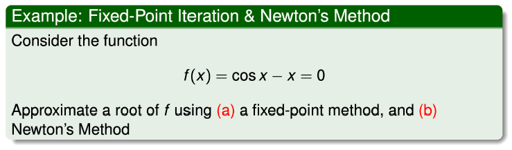
Example: Fixed Point Iteration & Newton's Method

Convergence using Newton's Method

Convergence using Newton's Method

Theoretical importance of the choice of $p_0$

• The Taylor series derivation of Newton's method points out the importance of an accurate initial approximation.
• The crucial assumption is that the term involving $\left(p-p_0\right)^2$ is, by comparison with $\left|p-p_0\right|$, so small that it can be deleted.
• This will clearly be false unless $p_0$ is a good approximation to $p$.
• If $p_0$ is not sufficiently close to the actual root, there is little reason to suspect that Newton's method will converge to the root.
• However, in some instances, even poor initial approximations will produce convergence.

  뉴턴의 방법의 테일러 급수 도출은 정확한 초기 근사치의 중요성을 지적한다.
  중요한 가정은 $\left(p-p_0\right)^2$와 관련된 용어가 $\left|p-p_0\right|$와 비교하여 너무 작아서 삭제할 수 있다는 것이다.
  $p_0$이 $p$에 대한 좋은 근사치가 아닌 한 이것은 분명히 거짓일 것이다.
  $p_0$이 실제 루트에 충분히 가깝지 않다면, 뉴턴의 방법이 루트로 수렴할 것이라고 의심할 이유가 거의 없다.
  그러나 어떤 경우에는 초기 근사치가 낮더라도 수렴이 발생할 수 있다.

Convergence Theorem for Newton's Method

• Let $f \in C^2[a, b]$. If $p \in(a, b)$ is such that $f(p)=0$ and $f^{\prime}(p) \neq 0$.
• Then there exists a $\delta>0$ such that Newton's method generates a sequence $\left\{p_n\right\}_{n=1}^{\infty}$, defined by

  $f \in C^2[a, b]$로 하자. $p \in(a, b)$가 $f(p)=0$ 및 $f^{\prime}(p) \neq 0$과 같은 경우.
  그런 다음 뉴턴의 방법이 다음과 같이 정의된 $\left\{p_n\right\}_{n=1}^{\infty}$ 시퀀스를 생성하도록 $\temp>0$이 존재한다.

converging to $p$ for any initial approximation

초기 근사치에 대해 $p$로 수렴

Convergence Theorem

• The proof is based on analyzing Newton's method as the functional iteration scheme $p_n=g\left(p_{n-1}\right)$, for $n \geq 1$, with

  증명은 $n \geq 1$에 대한 기능 반복 체계 $p_n=g\left(p_{n-1}\right)$로서 뉴턴의 방법을 분석하는 것에 기초한다.

• Let $k$ be in $(0,1)$. We first find an interval $[p-\delta, p+\delta]$ that $g$ maps into itself and for which $\left|g^{\prime}(x)\right| \leq k$, for all $x \in(p-\delta, p+\delta)$.

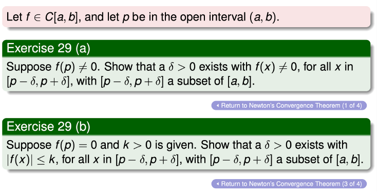
• Since $f^{\prime}$ is continuous and $f^{\prime}(p) \neq 0$, part (a) of Exercise 29 in Section $1.1$ - Ex29 implies that there exists a $\delta_1>0$, such that $f^{\prime}(x) \neq 0$ for $x \in\left[p-\delta_1, p+\delta_1\right] \subseteq[a, b]$.

  $k$를 $(0,1)$로 하자. 우리는 먼저 모든 $x \in(p-\delta, p+\delta)$에 대해 $g$가 자체 매핑되고 $\left|g^{\prime}(x)\right| \leq k$인 구간 $[p-\delta, p+\delta]$를 찾는다.
  $f^{\prime}$는 연속적이고 $f^{\prime}(p) \neq 0$이므로, 섹션 $1.1$ - Ex29의 부분 (a)은 $x \in\left[p-\delta_1, p+\delta_1\right] \subseteq[a, b]$.에 대해 $\delta_1>0$가 존재함을 의미한다.

• Thus $g$ is defined and continuous on $\left[p-\delta_1, p+\delta_1\right]$. Also

  따라서 $g$는 $\left[p-\delta_1, p+\delta_1\right]$에서 정의되고 연속적이다. 또한.

for $x \in\left[p-\delta_1, p+\delta_1\right]$, and, since $f \in C^2[a, b]$, we have $g \in C^1\left[p-\delta_1, p+\delta_1\right]$

• By assumption, $f(p)=0$, so

  $g^{\prime}(p)=\frac{f(p) f^{\prime \prime}(p)}{\left[f^{\prime}(p)\right]^2}=0$

• Since $g^{\prime}$ is continuous and $0<k<1$, part (b) of Exercise 29 in Section $1.1$ CEx23 implies that there exists a $\delta$, with $0<\delta<\delta_1$, and

  • $g^{\prime}$는 연속적이고 $0<k<1$이므로, 섹션 $1.1$ CEx23의 연습 29의 (b) 부분은 $0<\delta<\delta_1$인 $\delta$가 존재함을 암시한다.

• It remains to show that $g$ maps $[p-\delta, p+\delta]$ into $[p-\delta, p+\delta]$.
• If $x \in[p-\delta, p+\delta]$, the Mean Value Theorem chit implies that for some number $\xi$ between $x$ and $p,|g(x)-g(p)|=\left|g^{\prime}(\xi)\right||x-p|$. So

  $g$가 $[p-\delta, p+\delta]$를 $[p-\delta, p+\delta]$로 매핑한다는 것을 보여주는 것으로 남아 있다.
  $x \in[p-\delta, p+\delta]$인 경우 평균값 정리 키트는 $x$와 $p$ 사이의 일부 수 $\xi$에 대해 $|g(x)-g(p)|=\left|g^{\prime}(\xi)\right|x-p|$를 암시한다. 그래서

• Since $x \in[p-\delta, p+\delta]$, it follows that $|x-p|<\delta$ and that $|g(x)-p|<\delta$. Hence, $g$ maps $[p-\delta, p+\delta]$ into $[p-\delta, p+\delta]$.
• All the hypotheses of the Fixed-Point Theorem (Theorem24 are now satisfied, so the sequence $\left\{p_n\right\}_{n=1}^{\infty}$, defined by

  $x \in[p-\delta, p+\delta]$이므로 $|x-p|<\delta$와 $|g(x)-p|<\delta$가 뒤따른다. 따라서 $g$는 $[p-\delta, p+\delta]$를 $[p-\delta, p+\delta]$로 매핑한다.
  고정점 정리의 모든 가설(정리 24는 이제 만족되므로, $\left\{p_n\right\}_{n=1}^{\infty}$은 다음과 같이 정의된다.

converges to $p$ for any $p_0 \in[p-\delta, p+\delta]$.

모든 $p_0\in[p-\delta, p+\delta]$에 대해 $p$로 수렴한다.

Example 29, Section 1.1

Final Remarks on Practical Application

Choice of Initial Approximation

• The convergence theorem states that, under reasonable assumptions, Newton's method converges provided a sufficiently accurate initial approximation is chosen.
• It also implies that the constant $k$ that bounds the derivative of $g$, and, consequently, indicates the speed of convergence of the method, decreases to 0 as the procedure continues.
• This result is important for the theory of Newton's method, but it is seldom applied in practice because it does not tell us how to determine $\delta$.

  수렴 정리는 충분히 정확한 초기 근사가 선택된다면 합리적인 가정 하에서 뉴턴의 방법이 수렴한다고 말한다.
  또한 $g$의 도함수를 제한하고 결과적으로 방법의 수렴 속도를 나타내는 상수 $k$가 절차가 계속됨에 따라 0으로 감소한다는 것을 의미한다.
  이 결과는 뉴턴의 방법론에는 중요하지만 $\delta$를 결정하는 방법을 알려주지 않기 때문에 실제로 거의 적용되지 않는다.

In a practical application...

• an initial approximation is selected
• and successive approximations are generated by Newton's method.
• These will generally either converge quickly to the root,
• or it will be clear that convergence is unlikely.

  초기 근사치가 선택됨
  그리고 뉴턴의 방법에 의해 연속적인 근사치가 생성된다.
  이것들은 일반적으로 뿌리로 빠르게 수렴한다.
  그렇지 않으면 수렴 가능성이 낮다는 것이 분명해질 것이다.

Secant Method: Derivation & Algorithm

Rationale for the Secant Method

Problems with Newton's Method

• Newton's method is an extremely powerful technique, but it has a major weakness: the need to know the value of the derivative of $f$ at each approximation.
• Frequently, $f^{\prime}(x)$ is far more difficult and needs more arithmetic operations to calculate than $f(x)$.

  뉴턴의 방법은 매우 강력한 기술이지만 각 근사치에서 $f$의 도함수의 값을 알아야 한다는 주요 약점을 가지고 있다.
  종종 $f^{\prime}(x)$는 훨씬 어렵고 $f(x)$보다 계산하기 위해 더 많은 산술 연산이 필요하다.

Derivation of the Secant Method

Circumvent the Derivative Evaluation

If $p_{n-2}$ is close to $p_{n-1}$, then

Using this approximation for $f^{\prime}\left(p_{n-1}\right)$ in Newton's formula gives

This technique is called the Secant method

Secant Method: Using Successive Secants

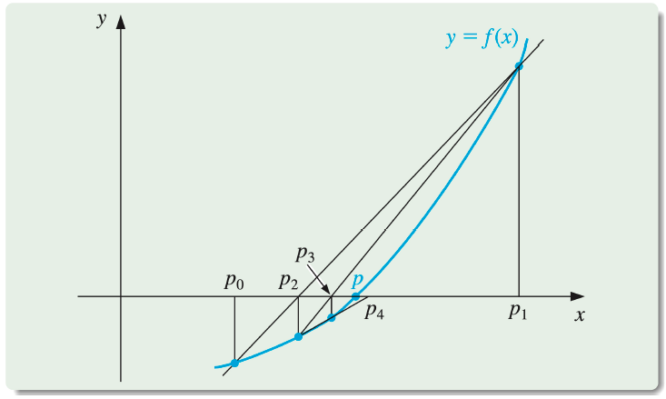
The Secant Method

Procedure

• Starting with the two initial approximations $p_0$ and $p_1$, the approximation $p_2$ is the $x$-intercept of the line joining $\left(p_0, f\left(p_0\right)\right)$ and $\left(p_1, f\left(p_1\right)\right)$.
• The approximation $p_3$ is the $x$-intercept of the line joining $\left(p_1, f\left(p_1\right)\right)$ and $\left(p_2, f\left(p_2\right)\right)$, and so on.
• Note that only one function evaluation is needed per step for the Secant method after $p_2$ has been determined.
• In contrast, each step of Newton's method requires an evaluation of both the function and its derivative.

  두 개의 초기 근사치 $p_0$ 및 $p_1$로 시작하는 근사치 $p_2$는 $\left(p_0, f\left(p_0\right)\right)$와 $\left(p_1, f\left(p_1\right)\right)$를 연결하는 선의 $x$ 절편이다.
  근사치 $p_3$는 $\left(p_1, f\left(p_1\right)\right)$와 $\left(p_2, f\left(p_2\right)\right)$를 연결하는 선의 $x$ 절편이다.
  $p_2$가 결정된 후에는 Secant 방법에 대해 단계당 하나의 함수 평가만 필요하다.
  이와는 대조적으로, 뉴턴의 방법의 각 단계는 함수와 그 도함수에 대한 평가를 필요로 한다.

The Secant Method: Algorithm

To find a solution to $f(x)=0$ given initial approximations $p_0$ and $p_1$; tolerance $T O L ;$ maximum number of iterations $N_0$.

1 Set $i=2, q_0=f\left(p_0\right), q_1=f\left(p_1\right)$
2 While $i \leq N_0$ do Steps 3-6:
3 Set $p=p_1-q_1\left(p_1-p_0\right) /\left(q_1-q_0\right)$. (Compute $\left.p_i\right)$
4 If $\left|p-p_1\right|<T O L$ then
OUTPUT $(p)$; (The procedure was successful.) STOP
5 Set $i=i+1$
6 Set $p_0=p_1 ; \quad\left(\right.$ Update $\left.p_0, q_0, p_1, q_1\right)$

7 OUTPUT ('The method failed after $N_0$ iterations, $N_0=$ ', $N_0$ ); (The procedure was unsuccessful) STOP

Comparing the Secant \& Newton's Methods

Example: $f(x)=\cos x-x$

Formula for the Secant Method

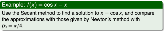
We need two initial approximations. Suppose we use $p_0=0.5$ and $p_1=\pi / 4$. Succeeding approximations are generated by the formula

Newton's Method for $f(x)=\cos (x)-x, p_0=\frac{\pi}{4}$

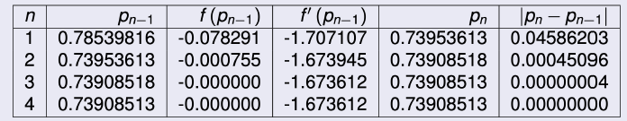
• An excellent approximation is obtained with $n=3$.
• Because of the agreement of $p_3$ and $p_4$ we could reasonably expect this result to be accurate to the places listed.

Secant Method for $f(x)=\cos (x)-x, p_0=0.5, p_1=\frac{\pi}{4}$

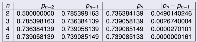
• Comparing results, we see that the Secant Method approximation $p_5$ is accurate to the tenth decimal place, whereas Newton's method obtained this accuracy by $p_3$.
• Here, the convergence of the Secant method is much faster than functional iteration but slightly slower than Newton's method.
• This is generally the case.

Order of Convergence of the Secant Method

Excersice 14, Section 2.4

Final Remarks

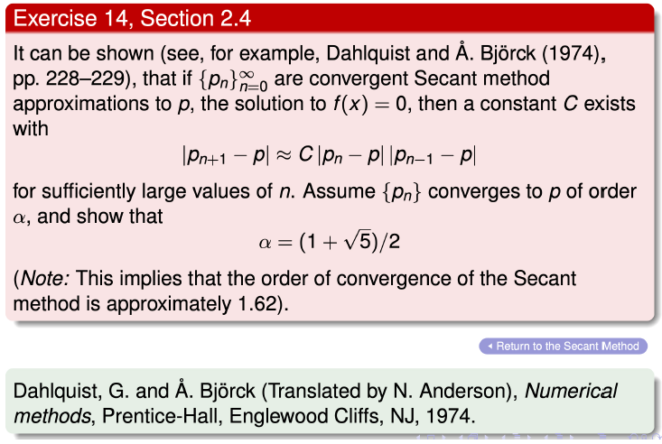
• The Secant method and Newton's method are often used to refine an answer obtained by another technique (such as the Bisection Method).
• Both methods require good first approximations but generally give rapid acceleration.

  세칸트 방법과 뉴턴의 방법은 종종 다른 기술(이분법)에 의해 얻어진 답을 정제하는 데 사용된다.
  두 방법 모두 좋은 첫 번째 근사치가 필요하지만 일반적으로 빠른 가속도를 제공한다.

The Method of False Position

The Method of False Position

Bracketing a Root

• Unlike the Bisection Method, root bracketing is not guaranteed for either Newton's method or the Secant method.
• The method of False Position (also called Regula Falsi) generates approximations in the same manner as the Secant method, but it includes a test to ensure that the root is always bracketed between successive iterations.
• Although it is not a method we generally recommend, it illustrates how bracketing can be incorporated.

Bisection Method와 달리, 루트 괄호는 Newton의 방법이나 Secant 방법에 대해 보장되지 않는다.
거짓 위치 방법(Regula Palsi라고도 함)은 세칸트 방법과 동일한 방식으로 근사치를 생성하지만 루트가 항상 연속 반복 사이에 괄호로 묶이는지 확인하는 테스트를 포함합니다.
일반적으로 권장하는 방법은 아니지만, 브래킷이 어떻게 통합될 수 있는지 보여줍니다.

Construction of the Method

• First choose initial approximations $p_0$ and $p_1$ with $f\left(p_0\right) \cdot f\left(p_1\right)<0$.
• The approximation $p_2$ is chosen in the same manner as in the Secant method, as the $x$-intercept of the line joining $\left(p_0, f\left(p_0\right)\right)$ and $\left(p_1, f\left(p_1\right)\right)$.
• To decide which secant line to use to compute $p_3$, consider $f\left(p_2\right) \cdot f\left(p_1\right)$, or more correctly $\operatorname{sgn} f\left(p_2\right) \cdot \operatorname{sgn} f\left(p_1\right)$ :
• If $\operatorname{sgn} f\left(p_2\right) \cdot \operatorname{sgn} f\left(p_1\right)<0$, then $p_1$ and $p_2$ bracket a root. Choose $p_3$ as the $x$-intercept of the line joining $\left(p_1, f\left(p_1\right)\right)$ and $\left(p_2, f\left(p_2\right)\right)$.
• If not, choose $p_3$ as the $x$-intercept of the line joining $\left(p_0, f\left(p_0\right)\right)$ and $\left(p_2, f\left(p_2\right)\right)$, and then interchange the indices on $p_0$ and $p_1$.

먼저 초기 근사치 $p_0$ 및 $p_1$을 $f\left(p_0\right) \cdot f\left(p_1\right)<0$로 선택한다.
근사치 $p_2$는 $\left(p_0, f\left(p_0\right)\right)$와 $\left(p_1, f\left(p_1\right)\right)$를 결합하는 선의 $x$ 절편으로서 Secant 방법과 동일한 방식으로 선택된다.
$p_3$을 계산하는 데 사용할 섹터 라인을 결정하려면 $f\left(p_2\right) \cdot f\left(p_1\right)$를 고려하거나 더 정확하게 $\operatorname{sgn} f\left(p_2\right) \cdot \operatorname{sgn} f\left(p_1\right)$를 고려해라.
-$\operatorname{sgn} f\left(p_2\right) \cdot \operatorname{sgn} f\left(p_1\right)<0$이면 $p_1$과 $p_2$는 루트를 괄호로 묶는다. $\left(p_1, f\left(p_1\right)\right)$와 $\left(p_2, f\left(p_2\right)\right)$를 결합하는 선의 $x$ 절편으로 $p_3$를 선택한다.
-그렇지 않으면 $\left(p_0, f\left(p_0\right)\right)$와 $\left(p_2, f\left(p_2\right)\right)$를 결합하는 선의 $x$-절편으로 $p_3$를 선택한 다음 $p_0$와 $p_1$의 인덱스를 교환한다.

Secant Method & Method of Flase Position

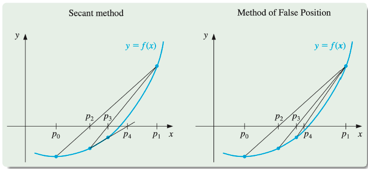
In this illustration, the first three approximations are the same for both methods, but the fourth approximations differ.

이 그림에서 처음 세 개의 근사치는 두 방법 모두에서 동일하지만 네 번째 근사치는 다릅니다.

The Method of False Position: Algorithm

To find a solution to $f(x)=0$, given the continuous function $f$ on the interval $\left[p_0, p_1\right]$ (where $f\left(p_0\right)$ and $f\left(p_1\right)$ have opposite signs) tolerance $T O L$ and maximum number of iterations $N_0$.

1 Set $i=2 ; q_0=f\left(p_0\right) ; q_1=f\left(p_1\right)$.
2 While $i \leq N_0$ do Steps 3-7:
3 Set $p=p_1-q_1\left(p_1-p_0\right) /\left(q_1-q_0\right)$. (Compute $\left.p_i\right)$
4 If $\left|p-p_1\right|<T O L$ then
OUTPUT $(p)$; (The procedure was successful): STOP
5 Set $i=i+1 ; q=f(p)$
6 If $q \cdot q_1<0$ then set $p_0=p_1 ; q_0=q_1$
7 Set $p_1=p ; q_1=q$
8 OUTPUT ('Method failed after $N_0$ iterations, $N_0=', N_0$ );
(The procedure was unsuccessful): STOP

The Method of False Position: Numerical Calculations

Comparison with Newton \& Secant Methods

Use the method of False Position to find a solution to $x=\cos x$, and compare the approximations with those given in a previous example which Newton's method and the Secant Method.

False Position의 방법을 사용하여 $x=\cos x$에 대한 솔루션을 찾고, 뉴턴의 방법 및 세칸트 방법이 이전 예에서 주어진 것과 근사치를 비교한다.

To make a reasonable comparison we will use the same initial approximations as in the Secant method, that is, $p_0=0.5$ and $p_1=\pi / 4$

합리적인 비교를 위해 우리는 세칸트 방법과 동일한 초기 근사치, 즉 $p_0=0.5$ 및 $p_1=\pi/4$를 사용할 것이다.

Comparison with Newton \& Secant Methods

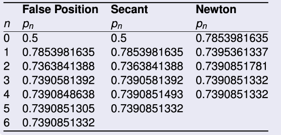
Note that the False Position and Secant approximations agree through $p_3$ and that the method of False Position requires an additional iteration to obtain the same accuracy as the Secant method.

거짓 위치와 세칸트 근사치는 $p_3$을 통해 일치하며, 거짓 위치의 방법은 세칸트 방법과 동일한 정확도를 얻기 위해 추가적인 반복이 필요하다는 점에 유의한다.

Final Remarks

• The added insurance of the method of False Position commonly requires more calculation than the Secant method,...
• just as the simplification that the Secant method provides over Newton's method usually comes at the expense of additional iterations.

허위포지션법의 추가보험은 일반적으로 세칸트법보다 더 많은 계산을 요한다.
세칸트 방법이 뉴턴의 방법에 대해 제공하는 단순화는 보통 추가적인 반복의 대가를 치르게 된다.

미분을 계산하려면 위와 같은 방식으로 근사하는 것이지, 실제 미분에 대한 데이터를 얻는 것은 어렵다.
p2. 뉴턴 메소드에서는 p0에서 접선을 그어서 p2를 구한다. p2의 위치가 더 오른쪽이다.
p0, p1은 선택해야 한다. initial 값이다.
f'을 모르기 때문에 두 개의 initial을 잡아서 선으로 연결하면 만나는 점이 p2이다.
p1, p2를 연결해서 만나는 점이 p3이다.
..
p3,p4를 연결해서 만나는 점이 p5이다.
n=10일 때 secant는 accurate.1.5배에서 1.7배 정도 느리다.
다른 것들보다는 매우 빠르지만, newton보다는 조금 느리다.
order : 차원이 다르다.
뉴턴과 일반 함수는 차원이 다르다.
보험을 드는 것이다. bracket 속에 root bracket is not guaranteed/
권장하는 방법은 아니다.