✍️ Abstract

A new method of representing 4D dynamic scenes as a mixture of static and dynamic voxels which utilizes the light weight static voxels for fast training and competitive rendering qualities.

🔒 Prerequisites

• Neural Radiance Fields
• Neural Voxel Fields
• Dynamic Nerf with multi-view inputs

🤔 Motivation

Different from Dynamic NeRF settings which takes input from a monocular camera, MixVoxels synthesizes vidos from real-world multi-view input first introduced by Nerual 3D Video Synthesis from Multi-view Video. Training models with such data is very time-consuming, hence MixVoxels, which speeds up training from days to 15~80 minuites.

📌 Main Method

MixVoxels have two main components which are the Voxel-grids (static and dynamic) for representation and a variation field for identifiying which points are static or dynamic.

1. Voxel-Grids

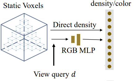
Static Voxel-grid

Static voxel-grid stores features about static scenes, invarying by time.

3D scene is split into

Density and color features are stored in these voxels

Density Feature : $\mathcal{S}^{\sigma} \isin \mathbb{R}^{N_x \times N_y \times N_z}$

Color Features : $\mathcal{S}^{c} \isin \mathbb{R}^{N_x \times N_y \times N_z \times C}$

As voxels corner positions are discrete, when sampling from contiuous positions, we interploate the features from nearest 8 positions.

Since colors depend on viewing point and are more complex features, we use a small MLP network $\mathcal{C}_\theta$

⚠️ keep in mind that there is no time query in static voxels as they are static.

Dynamic Voxel-grid

Dynamic vocel-grid stores features about dynamic scenes, varying by time.

• Dynamic Voxel-grid

Naively adding time dimension leads to big requirements in memory. Therefore authors propose a Spatialy Explicit and Temporaly Implicit representation.

3D scene is split into

Density and color features are stored in these voxels

Density Feature : $\mathcal{G}^{\sigma} \isin \mathbb{R}^{N_x \times N_y \times N_z\times C_1}$

Color Features : $\mathcal{G}^{c} \isin \mathbb{R}^{N_x \times N_y \times N_z \times C_2}$

Unlike Static grids, dynamic voxel grid features must have temperal information encoded, hence an additional dimension in density features.

These fetures are going to be queried by a time-aware projection, so in order to increase the feature dimension, authors imploy 2 MLPs $\mathcal{T}^{\sigma}_{\theta_1}$ and $\mathcal{T}^{c}_{\theta_2}$.

• Inner-product time query

For each time step $t$ there exists a learnable time-variant laten representation $\omega_t$ for quering time from features.

In summary, we can obtain density and color of a certain time step $t$ at point $(x,y,z$) and viewing direction $\bold{d}$ by

2. Variation Field

There are two voxel grids for representation. How do we know a given point is Static or Dynamic? → By a Variation Field

💡 Variation Field leverages pixel-level temporal variances of multi-view vidoes to estimate the voxel-level variances

Basically we meausre the pixel level temporal Variance as

Using pixel level temporal Variance, we estimate voxel-level variances by the following:

1) if pixel is static (blue ray) all voxels passing through blue ray is a static voxel

2) if pixel is dynamic (green ray) at least one of the voxels passing through a green ray is a dynamic voxel

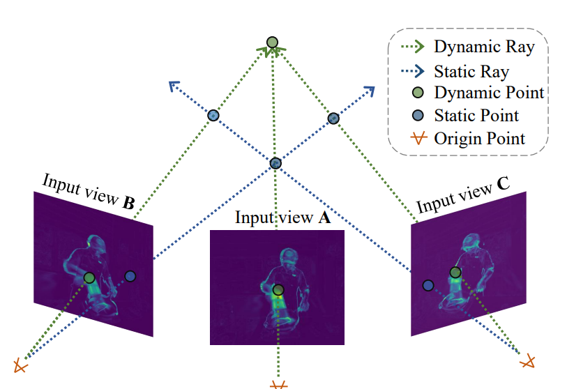
By the above process, we obtain a varaiation field

3. Inference

As we now know the which voxels are dynamic and static, we can split sampling poonts in the rays to ones that are dynamic and static.

1. From all the points sampled, use Static Voxels and render to recover mean pixel value
2. From only the dynmaic points, use dynamix Voxels to obtain density and color at time step $t$
3. Copy $\sigma, \bold{c}$ from static branch (for points that are static) and render them.

📋 Evaluation

MixVoxel’s contribution lies in the fast training time with comparable results.

Efficiency

MixVoxels achieve comparable results with much faster training time compared with DyNeRF and NeRFPlayer and less memory compared with Stream.

Quality

MixVoxels seem to have similar quality with DyNeRF but with 1/5000 to 1/1000 training time.

👻 Comments

• dynamic nerf들 최근 리서치를 보면 모두 dynamic과 static을 구분하는데 힘을 쏟는다.(d^2 nerf, nerfplayer, Mixvoxels) 결국 dynamic한 object들 보다static한 object들이 많다. 만약 dynamic한 부분들이 많은 scene들에 대해서는 artifact가 많을게 분명하다. 결국 dynamic한 부분보다 static한 부분이 많다는 inductive bias를 준거나 마찬가지이다.