CV 논문스터디 1주차

---

ImageNet Classification with Deep Convolutional Neural Networks

---

03/04 - 03/10

Abstract

Trained large, deep convolutional neural network to classify the 1.2 million high-resolution images into the 1000 different classes.

Neural Network Have 🙌

• 60 million parameters
• 650,000 neurons
  • 5 convolutional layers
    • some of max-pooling layers
  • 3 fully-connected layers ( final 1000-way softmax )

Neural Network Do 👍

• non-saturating neurons ( faster )
• efficient GPU implementation of the convolution operation ( faster )
• dropout ( reduce overfitting )

1. Introduction

To imporve object recognition performance

• collect larger datasets
• learn more powerful models
• use better techniques

Simple recognition tasks can be solved quite well with small datasets, especially if they are augmented with label-preserving transformations.

Objects in realistic settings exhibit considerable variability >> use larger training sets

Learn about many objects from images →
Need Model with large learning capacity ( immense complexity of object recognition ) →
Should also have lots of prior knowledge to compensate for all the data we don't have

• CNNs have much fewer connections and parameters
  • 👍 Easier to train
  • 👎 Performance is likely to be slightly worse

Problem is CNNs are prohibitively expensive to apply in large scale to high- resolution images. But! current GPUs, paired with a highly-optimized implementation of 2D convolution, are powerful enough to facilitate the training.

Specific contribution of this paper
They trained one of the largest convolutional neural networks to date on the subsets of ImageNet and achieved the best results ever reported.

Network Contains.. 📦

• A number of new and unusual features
  • improve its performance
  • reduce its training time
• Several effective techniques
  • prevent overfitting
• Five convolutional & three fully-connected layers
  • removing any convolutional layer resulted in inferior performance

🧑‍💼 : Results can be improved simply by waiting for faster GPUs and bigger datasets to become available..

2. The Dataset

ImageNet is a dataset of over 15 million labeled high-resolution images belonging to roughly 22,000 categories

Dataset 📀 : 1.2 million training images, 50,000 validation images, and 150,000 testing images

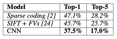
Need to report two error rates : top - 1 & top - 5

• top - 5 error rate = fraction of tests images for which the correct label is not among the five labels considered most probable by the model

Their system required a constant imput dimensionality >> down - sampled the images to a fixed resolution of 256 x 256.

Trained their network on the (centered) raw RGB values of the pixels

---

3. The Architecture

The architecture of network contains eight learned layers - 5 convolutional & 3 fully connected

3-1. ReLU Nonlinearity

Saturating nonlinearity (포화 비선형성) :
$f(x) = tanh(x)$ or $f(x) = (1 + e^{-x})^{-1}$
Non-Saturating nonlinearity (불포화 비선형성) :
$f(x) = max(0, x)$

Non-Saturating nonlinearity is faster than Saturating nonlinearity

ReLU = Rectified Linear Units
Deep convolutional neural networks with ReLUs train faster than with tanh units

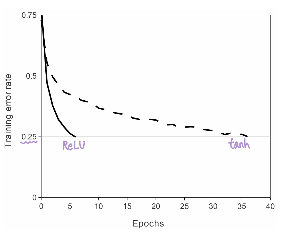
🧑‍💼 : Faster learning has a great influence on the performance of large models trained on large datasets.

3-2. Training on Multiple GPUs

Single GPU limits the maximum size of the networks that can be trained on it → Spread the net across two GPUs

🧑‍💼's Scheme |

• Put half of the kernels (or neurons) on each GPU
• GPUs communicate only in certain layers
  • Can precisely tune the amount of communication until it is an acceptable fraction of the amount of computation

Two-GPU net is faster to train than One-GPU net

3-3. Local Response Normalization

ReLU don't require input normalization to prevent them from saturating

Response-normalized activity :

• Denoting by the activity of neuron (computed by applying kernal $i$ at position $(x,y)$)
  ⬇️

• Applying the ReLU nonlinearity

  $b_{x,y}^i= a_{x,y}^i / (k + α\displaystyle\sum_{j= max(0,i-n/2)}^{\min(N-1,i+n/2)}{(a_{x,y}^j)^2})^β$
  • $n$ = adjacant kernel maps
  • $N$ = total number of kernels in the layer
  • $k, n, α, β$ = hyper - parameters
    • $k=2, n=5, α=10^{-4}, β=0.75$
  • Ordering of the kernel maps = abritrary & determined before training begins

Response Normalization creates competition for big activities amongst neuron outputs computed using different kernels

Apply the ReLU nonlinearity in certain layers >> Apply this normalization

🧑‍💼 : Ours would be termed "brightness normalization", since we do not substract the mean activity

3-4. Overlapping Pooling

Pooling layers in CNNs summarize the outputs of neighboring groups of neurons in the same kernel map.

$s$ = How far apart the pooling units are placed ($s$ pixels)
$z$ = The size of the neighborhood that each pooling unit observes ($z$ x $z$ pooling units)

• $s = z$, obtain traditional local pooling as commonly employed in CNNs
• $s < z$, obtain overlapping pooling

🧑‍💼 : We used, $s = 2, z = 3$. Models with overlapping pooling find it slightly more difficult to overfit

3-5. Overall Architecture

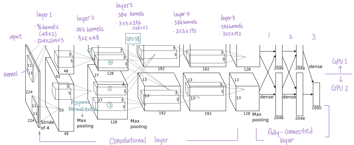
Net contains 8 layers with weights.

• Layer 1~5 : convolutional layer
• Layer 6~8 : fully-connected
• Output : Fed to a 1000-way softmax which produces a distribution over the 1000 class labels

Maximizing the multinomial logistic regression objective =
Maximizing the average across training cases of the log-probability of the correct label under the prediction distribution

• Kernels of Conv Layer 2, 4, 5
  • Connected only to those kernel maps in the previous layer which reside on the same GPU (3.2 training on Multiple GPUs)
• Kernels of Conv Layer 3
  • Connected to all kernel maps in the second layer
• Neurons in the fully-connected layers
  • Connected to all neurons in the previous layer

• Conv Layer 1 → ReLU → Response Normalization → Max Pooling → Conv Layer 2
• Conv Layer 2 → ReLU → Response Normalization → Max Pooling → Conv Layer 3
• Conv Layer 3 → ReLU → Conv Layer 4
• Conv Layer 4 → ReLU → Conv Layer 5
• Conv Layer 5 → ReLU → Max Pooling → Fully-connected Layer

---

4. Reducing Overfitting

🧑‍💼 :Our neural network architecture has 60 million parameters

4-1. Data Augmentation

To reduce overfitting on image data : Artificially enlarge the dataset using label-preserving transformations

🧑‍💼 : Two distinct forms of data augmentation is employed

Both allow transformed images to be produced from the original with very little computation → don't need to be stored on disk

(1) Generating image translations and horizontal reflections

Extract random 224 x 224 patches & their horizontal reflections from the 256 x 256 images → Train network on these extracted patches.

At test time, the network makes a prediction by extracting five 224 x 224 patches (4 corner + 1 center) + their horizontal reflections = 10 patches. And average the predictions made by the network's softmax layer on the 10 patches

(2) Altering the intensities and horizontal reflections

For training image, Add multiples of the found principal components with magnitudes proportional to the corresponding eigenvalues times a random variable drawn from $X$ ~ $N(0, {(0.1)}^2)$, they add the following quantity : $[p_1,p_2,p_3][α_1λ_1, α_2λ_2 , α_3λ_3 ]^T$

• $p_i$ & $λ_i$ : $i$th eigenvector and eigenvalue of the 3 x 3 covriance matrix of RGB pixel values
• $α_i$ : aforementioned random variable. Each $α_i$ is drawn only once for all the pixels of a particular training image until that image is used for training again.

4-2. Dropout

To reduce test errors : Combining the predictions of many different models → EXPENSIVE!

Dropout : Consists of setting to zero the output of each hidden neuron with probability 0.5

• The "dopped out" neuron don't contribute to the forward pass and don't participate in back-propagation.

Dropout reduces complex co-adaptations of neurons,since a neuron cannot rely on the presence of particular other neurons → Forced to learn more rubust features that are useful in conjunction with many different random subsets of the other neuron

5. Details of learning

Trained models using stochastic gradient descent with a batch size of 128 examples, momemtum of 0.9, and weight decay of 0.0005

Weight decay : Reduces the model's training error

• $v_{i+1} := 0.9 ⋅ v_i - 0.0005 ⋅ ϵ ⋅ w_i - ϵ ⋅ <{∂L\over∂w }|_{w_i}>_{D_i}$
• $w_{i+1} := w_i + v_{i+1}$
  • $i$ : iteration index
  • $v$ : momentum variable
  • $ϵ$ : learning rate
  • $<{∂L\over∂w }|_{w_i}>_{D_i}$ : average over the $i$th gatch $D_i$ of the derivative of the objective with respect to $w$, evaluated at $w_i$

• Initialized the weights in each layer from $X$ ~ $N(0, {(0.1)}^2)$
• Initialized the neuron biases in the second, fourth, and fifth convolutional layers, as well as in the fully-connected hidden layers, with the constant 1. And the remaining layers with the constant 0
  → Accelerates the early stages of learning by providing the ReLUs with positive inputs

🧑‍💼 : We trained the network for rougly 90 cycles through the training set of 1.2 million images, which took five to six days on two NVIDIA GTX 580 3GB GPUs.

---

6. Results

6-1. Qualitative Evaluations

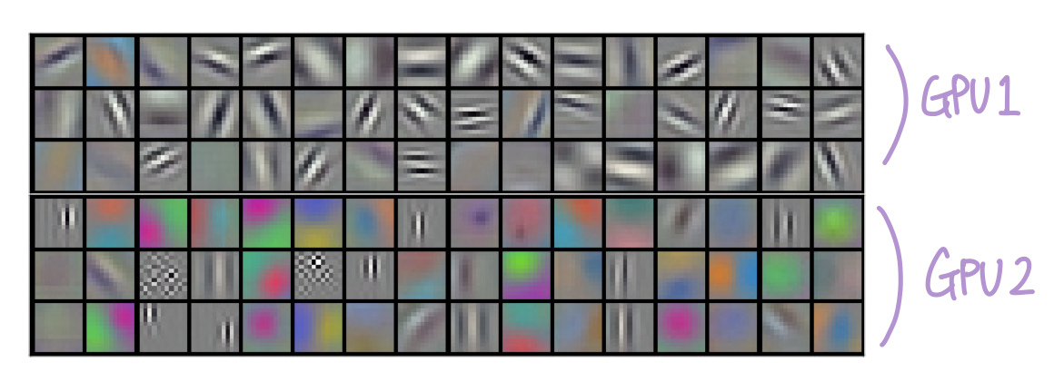
^ Convolutional kernels learned by the network's two data-connected layers

• Kernels on GPU 1 : largely color-agnostic
• Kernels on GPU 2 : largely color-specific

Specialization occurs during every run and is independent of any particular random weight initialization.

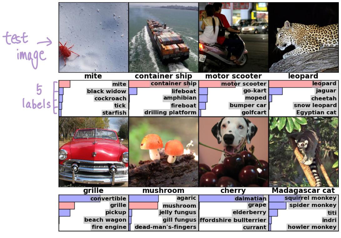
^ What the network has learned by computing its top-5 predictions on eight test images
🧑‍💼 : Even off-center objects can be recognized by the net

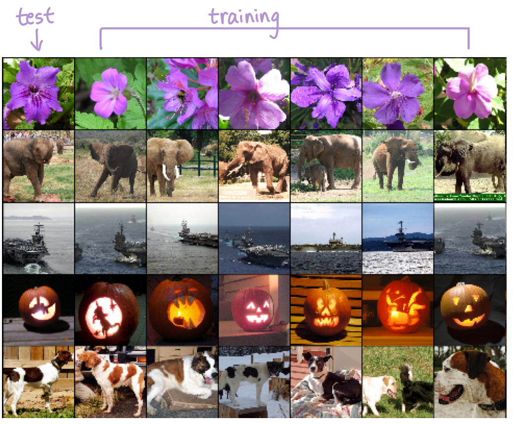
Probe the network's visual knowledge is to consider the feature activations induced by and image at the last, 4096-dimensional hidden layer.

🧑‍💼 : At the pixel level, the retrieved training images are generally not close in L2 to the query images in the first column. (Retrieved dogs and elephants appear ina variety of poses)

Computing similarity by using Euclidean distance between two 4096-dimensional, real-valued vectors is inefficient
BUT! it could be made efficient by training an auto-encoder to compress these vectors to short binary codes

7. Discussion

Network's perfomance degrades if a single convolutional layer is removed. So depth really is important for achieving results.

🧑‍💼 : We did not use any unsupervised pre-training even though we expect that it will help. But we still have many orders to go in order to match the infero-temporal pathway of the human visual system.

---