CV 논문스터디 4주차

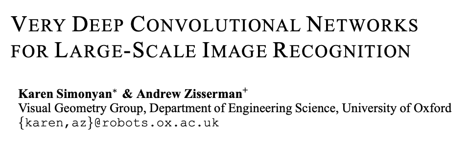
Very Deep Convolutional Networks For Large-Scale Image Recognition

---

Abstract

We investigate the effect of the convolutional network depth on its accuracy in the large-scale image recognition setting.

Main contribution is a thorough evaluation of networks of increasing depth using an architecture with very small (3x3) convolutional filters.

1. Introduction

ConvNet이 성공하고 나서, 이를 improve하려는 움직임이 많아졌다.

• To achieve better accuracy
  • Utilize smaller receptive window size and smaller stride of the first convolutional layer (더 작은 window size & convolutional layer)
  • Training and testing the networks densely over the whole image and over multiple scales (더 밀집된 사진 & 다수의 scale)

🧑‍💻 : We address another important aspect of ConvNet architecture design - its depth
We fix other parameters of the architecture, and steadily increase the depth of the network by adding more convolutional layers.
→ 모든 layer에 굉장히 작은 convolution filter(3x3)를 사용하기 때문에 가능하다.

결과적으로,

• Achieved state-of-the-art accuracy on ILSVRC classification and localisation tasks
• Applicable to other image recognition datasets
  • Achieved excellent performance even when used as a part of a relatively simple pipelines

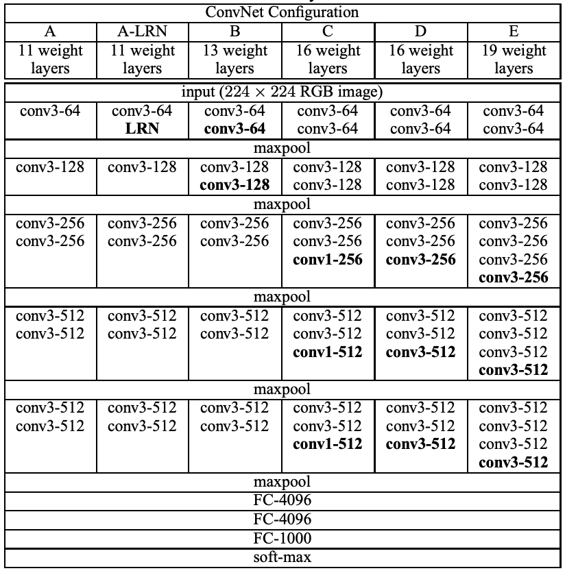
2. ConvNet Configurations

All our ConvNet layer configurations are designed using the same principles.

2-1. Architecture

ConvNet의 아키텍처를 설명했다.

CNN (Convolutional Neural Network)
(1주차에 배웠음)

• 핵심 개념
  • Convolution ( 합성곱 연산 )
    • 필터(Filter, Kernel)를 이용해 특징을 추출
    • FCN과 달리, 공간적 구조를 유지
  • Pooling ( 풀링 )
    • 특징 맵의 크기를 줄여 연산량을 감소시키고, 중요한 정보만 유지하는 과정
  • Activation Function ( 활성화 함수 )
    • ReLU(Rectified Linear Unit)가 일반적으로 사용됨
  • Fully Connected Layer ( 완전연결층 )
    • 추출된 특징을 기반으로 분류(Classification)를 수행

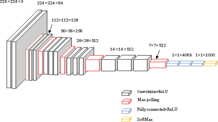
Trainig을 할 때, input은 224x224 RGM image로 고정을 했다.
Pre-processing은 평균 RGB 값을 빼는 것이 었다. 이것은 각각의 픽셀마다 training set에서 계산되었다.
이미지는 Convolutional layer 더미를 지나갔는데, 우리는 3x3 receptive field를 사용하였다.
배치들 중 하나에는 1x1 convolution filter를 활용하였다. 이것은 인풋 채널의 linear transformation으로 보일 수 있다.
Convolution stride는 1 pixel로 고정되어있다.
Spatial pooling은 5개의 max-pooling layers로 이루어진다. max-pooling layer는 2x2 pixel 윈도우에 stride 2로 수행된다.
Convolution layer 더미는 3개의 Fully-Connected layer 앞에 있다.
마지막 layer는 soft-max layer 이다. 보통 VGGNet에서는 Conv → Conv → Max-pooling 구조가 반복되고, 마지막에 Fully-Connected 층이 배치된다.

모든 숨겨진 layer들은 ReLU로 되어있다.
어떤 네트워크도 LRN normalization을 포함하지 않는데, 이것은 이러한 Normalization이 ILSVRC 데이터셋에서 어떠한 성능 개선을 하지 않고, 메모리 소비와 계산 시간만 늘렸기 때문이다.

2-2. Configurations

2-3. Discussion

We use very small 3 x 3 receptive fields throughout the whole net, which are convolved with the input at every pixel with stride 1.

단일 7x7 layer 대신, 3개의 3x3 convolutional layer를 사용해서 얻은 장점

• We incorporate three non-linear rectification layers instead of a single one
  • Made decision function more discriminative
• We decrease the number of parameters
  • 이것은 7x7 conv. filters에 정규화를 도입한 것처럼 보인다
  • 3x3 filters들을 통한 decomposition을 촉진하면서

The incorporation of 1x1 conv. layers is a way to increase the non-linearity of the decision function without affecting the receptive fields of the conv. layers
= 1x1 컨볼루션 레이어를 도입하는 것은 컨볼루션 레이어의 수용 영역(receptive field)에 영향을 주지 않으면서 결정 함수의 비선형성을 증가시키는 방법이다.

즉, 1x1 필터가 각 픽셀을 독립적으로 처리하기 때문에 기존의 수용 영역 크기를 유지하면서, 더 복잡한 변환을 할 수 있다

Small size convolution filter는 이전에도 사용되었다.
GoogLeNet은 우리의 작업과 독립적으로 발전되었지만, deep ConvNet을 기반으로 한다는 것과 small convolution filters를 사용한다는 점에서 닮아있다. 하지만 GoogLeNet이 더 복잡하고, 계산량을 줄이기 위해 특징 map의 spatial resolution이 첫번째 레이어에서 굉장히 공격적으로 줄어들었다.

3. Classification Framework

We describe the details of classification ConvNet training and evaluation

3-1. Training

The training is carried out by optimizing the multinomial logistic regression objective using mini-batch gradient descent with momentum.

We conjecture that in spite of the larger number of parameters and the greater depth of our nets compared to AlexNet, the nets required less epochs to converge due to (a) implicit regularization imposed by greater depth and smaller conv. filter sizes; (b)pre-initialization of certain layers
: 깊고 복잡한 네트워크라도 더 적은 에포크로 빠르게 학습될 수 있다. 그 이유는 (a) 암묵적 정규화 효과, (b) 사전 초기화 때문이라고 추측한다.

Implicit regularization (암묵적 정규화)
: 명시적으로 정규화 기법을 적용하지 않아도 학습 과정 자체가 정규화 역할을 수행하는 현상
→ 네트워크 아키텍처나 최적화 기법에 따라 자동으로 발생할 수 있다

Pre-initialization (사전 초기화)
: 신경망 학습을 시작하기 전에 가중치를 적절히 초기화하여 학습이 원활하게 진행되도록 하는 기법

We found that it is possible to initialize the weights without pre-training by using the random initialization procedure
= 우리는 사전 학습(pre-training) 없이도 랜덤 초기화 절차를 사용하여 가중치를 초기화하는 것이 가능하다는 것을 발견했다

Training image size

We consider 2 approaches for setting the training scale S

• Fix S = single-scale training
  • 이미지에서 특정영역을 잘라도, 포함된 정보는 여전히 다양한 크기를 유지한다
• multi-scale training (= scale jittering)
  • $[S_{min},S_{max}]$ 사이의 사이즈로 랜덤하게 S를 rescale 한다
    • 논문의 경우 [256 , 512]

scale jittering
: Data augmentation 중 하나로, 학습 중 이미지의 크기를 무작위로 변환하여 모델의 일반화 성능을 향상시키는 방법

For speed reasons, we trained multi-scale models by fine-tuning all layers of a single-scale model with the same configuration, pre-trained with fixed S = 384.
속도상의 이유로, 우리는 단일 스케일 모델을 S = 384로 고정하여 사전 학습한 후, 동일한 구성으로 모든 레이어를 fine-tuning하여 다중 스케일 모델을 학습했다.

3-2. Testing

It is isotropically resclaed to a pre-defined smallest image side, denoted as Q (test scale ).
The network is applied densely over ther rescaled test image in a way similar to OverFeat.
The resulting fully-convolutional net is then applied to the whole image.
To obtain a fixed-size vector of class scores for the image, the class score map is spatially averaged (sum-pooled).
= VGGNet의 테스트 방식은 이미지를 사전 정의된 크기로 조정하고, 그 조정된 이미지를 밀집하게 네트워크에 적용한 후, 합 풀링을 통해 최종 클래스 점수 벡터를 얻는 방식

OverFeat (2014)
: 분류, 탐지, 위치 추정을 동시에 해결하는 모델로, 이전의 모델들과 비교하여 다중 작업을 하나의 네트워크에서 처리할 수 있도록 구성하였다.

Since, the fully-convolutional network is applied over the whole image, there is no need to sample multiple crops at test time AlexNet, which is less efficient as it requires network re-computation for each crop.
: VGGNet은 전체 이미지를 한 번에 처리할 수 있기 때문에, 각각의 이미지 패치를 처리하기 위해 네트워크를 반복적으로 계산하는 AlexNet보다 효율적

3-3. Implementation Details

Multi-GPU training exploits data parallelism, and is carried out by splitting each batch of training images into several GPU batches, processed in parallel on each GPU. Gradient computation is synchronous across the GPUs, so the result is exactly the same as when training on a single GPU.

= 멀티 GPU 훈련은 데이터 병렬성을 활용하며, 훈련 이미지의 각 배치를 여러 GPU 배치로 나누어 각 GPU에서 병렬로 처리한다. 그래디언트 계산은 GPU 간에 동기화되므로, 결과적으로 단일 GPU에서 훈련할 때와 정확히 동일한 결과가 도출된다.

4. Classification Experiments

Dataset
🧑‍💻 : We present the image classification results

Dataset includes..

• training (1.3M images)
• validation (50K images)
• testing (100K images )

Performance is evaluated..

• top-1 error
  • multi-class classification error
• top-5 error
  • Computed as the proportion of images such that the ground-truth category is outside the top-5 predicted categories

For the majority of experiments, we used the validation set as the test set.

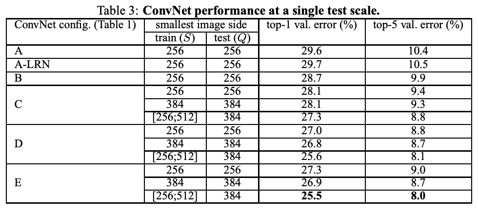
4-1. Single Scale Evaluation

Test image size :

• Q = S for fixed S
• Q = 0.5($S_{min} + S_{max}$) for jittered $S$ ∈ [$S_{min} ,S_{max}$]

1. Using local response normalization (A-LRN network) does not improve on the model A without any normalization layers

2. Classification error decreases with the increased ConvNet depth
   → while the additional non-linearity does help, it is also important to capture spatial context by using conv. filters with non-trivial receptive fields

   non-trivial receptive field
   : 모델이 입력 이미지에서 더 넓은 영역을 보게 되는 과정을 통해, 더 복잡하고 유용한 특징을 학습할 수 있게 만드는 것

   Deep net with small filters outperforms a shallow net with larger filters

3. Scale jittering at training time leads to significantly better results than training on images with fixed smallest side
   → training set augmentation by scale jittering is indeed helpful for capturing multi-scale image statistics

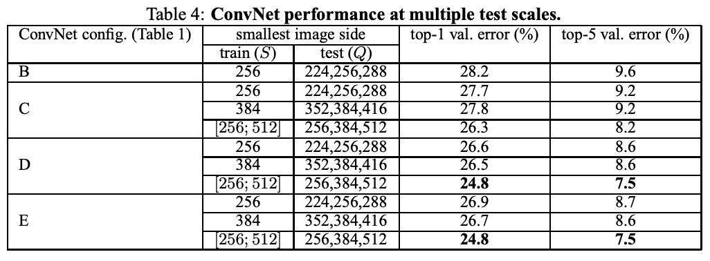
4-2. Multi-Scale Evaluation

Now assess the effect of scale jittering at test time.
It consists of running a model over several rescaled versions of a test image, followed by averaging the resulting class posteriors.

Fixed S

• test와 train 사이의 large discrepancy(performance drop)를 줄이기 위해!
  • $Q =$ {$S-32, S, S+32$}

Scale jittering

• 테스트에 더 넓은 크기 가능!
  • $Q =$ {$S_{min}, 0.5(S_{min}+S_{max}), S_{max}$}

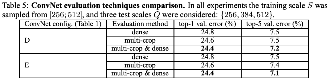
4-3. Multi-Crop Evaluation

Assess the complementarity of the two evaluation techniques by averaging their soft-max outputs

Soft-Max
: 여러 개의 클래스 중에서 가장 가능성이 높은 클래스를 선택하는 함수

• 출력을 확률 분포 (합이 1이되는 형태) 로 변환해줌
• 딥러닝의 다중 클래스 분류 문제에서 마지막 층 (출력층) 에 주로 사용됨

Multiple crops perform slightly better than dense evaluation, and the two approaches are indeed complementary. All due to a different treatment of convolution boundary conditions

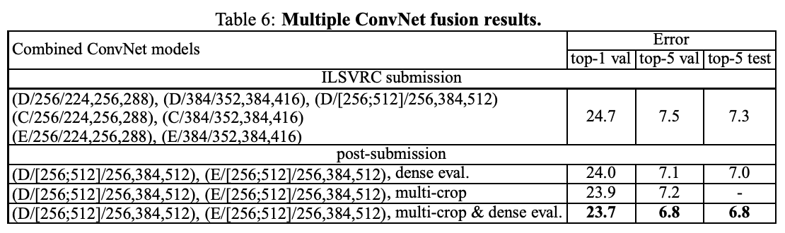
4-4. ConvNet Fusion

Combine the outputs of several models by averaging their soft-max class posteriors. This improves the performance due to complementarity of the models.

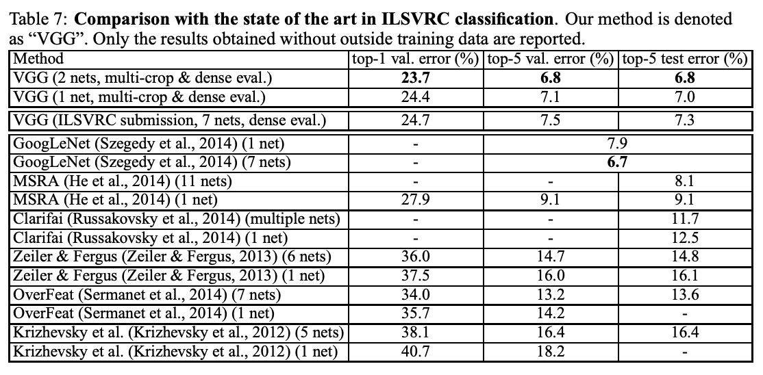
4-5. Comparison with the State Of The Art

We compare our results with the state of the art (GoogLeNet).

Our best result is achieved by combining just two models.
We did not depart from the classical ConvNet architecture of ConvNet, but imporved it by substantially increasing the depth

5. Conclusion

Evaluated very deep convolutional networks for large-scale image classification.

Representation depth is beneficial for the classification accuracy, and that state-of-the-art performance on the ImageNet challenge dataset can ba achieve using a conventional ConvNet architecture with substantially increased depth.

→ ConvNet(합성곱 신경망)의 깊이를 크게 늘리면, ImageNet 데이터셋에서 최신 기술 수준의 성능을 얻을 수 있다

---

A. Localisation

In this section, we turn to the localization task of the challenge. It can be seen as a special case of object detection, where a single object bounding box should be predicted for each of the top-5 classes, irrespective of the actual number of objects of the class.
→ 실제 객체의 개수와 관계없이 각 상위 5개 클래스에 대해 하나의 객체 경계 상자를 예측해야 한다

A-1. Localisation ConvNet

We use a very deep ConvNet, where the last fully connected layer predicts the bounding box location instead of the class scores. A bounding box is represented by a 4-D vector storing its center coordinates, width, and height
→ 마지막 완전 연결층은 클래스 점수 대신 경계 상자 위치를 예측한다. 경계 상자는 중심 좌표, 너비, 높이를 저장하는 4차원 벡터로 표현된다

There is a choice,

• the bounding box prediction is shared across all classes
  • last layer is 4-D
• the bounding box prediction is class-specific
  • last layer is 4000-D

Apart from the last bounding box prediction layer, we use the ConvNet architecture D, which contains 16 weight layers.

Training
We replace the logistic regression objective with a Euclidean loss, which penalises the deviation of the predicted bounding box parameters from the ground-truth.

Testing
We consider two testing protocols

• Used for comparing different network modifications on the validation set, and considers only the bounding box prediction for the ground truth class

• Fully-fledged, testing procedure is based on the dense application of the localization ConvNet to the whole image, similarly to the classification task.

  • instead of the class score map, the output of the last fully-connected layer is a set of bounding box predictions.
  • Final prediction, we utilize the greedy merging procedure box predictions.

Greedy merging procedure (탐욕적 병합 절차)
: 두 개 이상의 요소를 합칠 때, 매번 가장 작은 (혹은 가장 큰) 항목을 선택하여 병합하는 방식

A-2. Localisation Experiments

In this section, we first determine the best-performing localization setting, and then evaluate it in a fully-feldged scenario.
The localisation error is measured according to the ILSVRC criterion

• Settings comparision
  • per-class regression (PCR) outperforms the class-agnostic single-class regression (SCR)
  • Fine-tuning all layers for the localisation task leads to noticeably better results than fine-tuning only the fully-connected layers
• Fully-fledged evaluation
  • We now apply PCR in the fully-fledged scenario
  • Application of the localisation ConvNet to the whole image substantially improves the results compared to using a center crop.
  • Similary to the classification task, testing at several scales and combining the predictions of multiple networks further improves the performance.
• Comparision with the state of the art
  • We compare our best localisation result with the state-of-the-art.
  • We got better results with a simpler localisation method, but a more powerful representation

B. Generalisation Of Very Deep Features

We evaluate our ConvNets, pre-trained on ILSVRC, as feature extractors on other, smaller, datasets, where training large models from scratch is not feasible due to overfitting.
→ 우리는 ILSVRC에서 미리 학습된 ConvNet을 다른 작은 데이터셋에서 특징 추출기로 평가합니다. 작은 데이터셋에서는 큰 모델을 처음부터 학습하는 것이 과적합문제로 인해 실행 불가능하기 때문입니다.

We consider two models with the best classification performance on ILSVRC - configurations "Net-D" and "Net-E"

To utilise the ConvNet for image classification on other datasets, we remove the last fully-connected layer and use 4096-D activations of the penultimate layer as image features.
→ ConvNet 모델을 다른 데이터셋에 적용하기 위해 마지막 층을 제거하고, 그 이전 층에서 나온 특징을 사용하여 이미지를 분류하는 방법

An image is first rescaled so that its smallest side equals Q, and then the network is densely applied over the image plane, then perform global average pooling on the resulting feature map.
→ 이미지를 전처리한 후, 네트워크가 이미지 평면 전체에 밀집하게 적용되고, 마지막으로 특징 맵에서 글로벌 평균 풀링을 수행

We extract features over several scales Q. We also assess late fusion of features, computed using two networks, which is performed by stacking their respective image descriptors.

→ 다양한 스케일에서 특징을 추출하고, 두 개의 네트워크에서 나온 특징을 결합하는 후처리 방법

descriptor
: 어떤 객체나 데이터를 나타내는 특성이나 속성

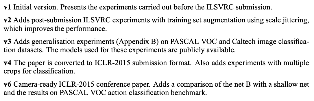
C. Paper Revisions