CV 논문스터디 3주차

Rethinking the Inception Architecture for Computer Vision

---

Abstract

💁 : We are exploring ways to scale up networks in ways that aim at utilizing the added computation as efficiently as possible by suitably factorized convolutions and aggressive regularization

1. Introduction

Since Alexnet has been successfully applied to a larger variety of computer vision tasks, these successes spurred a new line of research that focused on finding higher performing convolutional neural networks.

Gains in the classification performance tend to transfer to significant quality gains in a wide variety of application domains.

• Architectural improvements in deep convolutional architecture
  • Utilized for improving performance for most other computer vision tasks that are increasingly reliant on high quality, learned visual features
• Improvements in the network quality
  - New application domains for convolutional networks in cases where AlexNet features could not compete with hand engineered, crafted solutions

VGGNet
👍 Compelling feature of architectural simplicity
👎 High cost → evaluating the network requires a lot of computation

---

GoogLeNet
👍 Perform well even under strict constraints on memory and computational budget

Inception이 계산 비용이 훨씬 낮기 때문에, 모바일 비전처럼 메모리나 계산 수용력이 제한되어 있는 빅데이터 시나리오에서 많이 사용되었다.

However Utilizing Inception networks add extra complexity + widen the efficiency gap.

If the architecture is scaled up naively, large parts of the computational gains can be immediately lost.

💁 : In this paper, we start with describing a few general principles and optimization ideas that that proved to be useful for scaling up convolution networks in efficient ways.
This is enabled by the generous use of dimensioanl reduction and parallel structures of the Inception modules which allows for mitigating the impact of structural changes on nearby components.

2. General Design Principles

A few design principles based on large-scale experimentation with various architectural choices with convolutional networks.

1. Avoid representational bottlenecks

Representational bottleneck
: 뉴럴 네트워크가 정보를 너무 압축하여 중요한 특징을 잃어버리는 현상
: 특정 레이어에서 특징을 효과적으로 표현하지 못해서 학습이 제한되는 현상

In general, the representation size should gently decrease from the inputs to the outputs before reaching the final representation used for the task at hand.

단순히 차원의 수가 많다고 해서 반드시 많은 정보를 가지고 있는 것은 아니다. Correlation structure같은 중요한 요인을 버렸을 때, 저런 현상이 일어나는 것!

2. Higher dimensional representations are easier to process locally within a network

Increasing the activations per tile in a convolutional network → More disentangled features → Train faster
= 활성화 함수 증가 → 분리된 특징 추출 가능 → 트레이닝 빨라짐

3. Spatial aggregation can be done over lower dimensional embeddings without much on any loss in representational power

Spatial aggregation (공간 응집)
: 이미지나 공간 데이터에서 주변 값들을 합쳐 정보를 요약하거나 처리하는 과정
→ 주변 환경을 통해 정보를 처리하는 것!

During dimension reduction → Strong correlation between adjacant unit results in much less loss of information
게다가! dimension reduction → 속도도 빨라짐

4. Balance the width and depth of the network

Optimal performance : balancing the number of filters per stage & the depth of the network

The optimal improvement for a constant amount of computation can be reached if both are increased in parallel.

💁 : The idea is to use them judiciously in ambiguous situations only.
위의 아이디어들은 다 맞는 말이긴 한데, 언제나 quality를 올려주는 건 아니기 때문에, 신중하게 사용하는 것이 좋다~

3. Factorizing Convolutions with Large Filter Size

Factorizing Convolution
: 큰 커널을 두 개 이상의 작은 커널로 분해하여 연산을 더 효율적으로 수행하는 기법
ex) 3x3 → 1x1 이전 논문!!

In a vision network , it is expected that the outputs of near-by activations are highly correlated. Therefore, we can expect that their activations can be reduced before aggregation and that this should result in similarly expressive local representations.

aggregate(통합)하기 전에, 이미 highly correlated하니까 줄일 수 있지 않을까? > 이걸 비슷하게 표현되는 로컬 표현들에 적용될 수 있겠다~

Here we will explore other ways of factorizing convolutions in various settings, especially in order to increase the computational efficiency of the solution.

특히 계산 효율성을 증가시키면서, 다양한 환경에서 factorizing convolution을 할 수 있는 다른 방법을 찾아보겠다 !

< 한국어 번역 >
Inception networks 는 fully convolutional 하기 때문에
→ 각각의 가중치 = 활성화 함수에 대한 하나의 곱셈연산 ( weight = 1x1 convolution )
= 계산 비용 감소하려는 시도 → 파라미터 수의 감소
= suitable factorization (적절한 인수분해) → more disentangled parameters (더 분해된 parameter) → training이 빨라진다
또한, save된 계산 & 메모리를, 장점(하나의 컴퓨터에서 병렬 훈련을 할 수 있음 = 리소스 제약이 있을 때 효율적임)을 유지하면서, 네트워크의 filter-bank size를 증가시키는 데 사용 가능

3-1. Factorization into smaller convolutions

Convolutions with larger spatial filters tend to be disproportionally expensive in terms of computation.

However, we can ask whether a 5 x 5 convolution could be replaced by a multi-layer network with less parameters with the same input size and output depth.

Since we are constructing a vision network, it seems natural to exploit translation invariance again and replace the fully connected component by a two layer convolutional architecture ( 5x5 → 2개의 3x3 )

translation invariance
: 입력 이미지나 데이터가 위치가 바뀌어도 모델이 동일한 출력을 내는 성질

Sliding this small network over the input activation grid boils down to replacing the 5 x 5 convolution with two layers of 3 x 3 convolution
→ This setup clearly reduces the parameter count by sharing the weights between adjacant tiles.

The expected computational cost savings : $n = αm$
→ we want to change the number of activations/unit by a constant alpha factor
(α is typically slightly larger than 1)

Still, this setup raises two general questions :

• Does this replacement result in any loss of expressiveness?
• If our main goal is to factorize the linear part of the computation, would it not suggest to keep linear activations in the first layer?

→ Using linear activation was always inferior to using rectified linear units in all stages of the factorization.

큰 필터(5×5, 7×7)를 작은 필터(3×3) 여러 개로 나누면 연산량을 줄이고 표현력도 증가한다.

3-2. Spatial Factorization into Asymmetric Convolutions

Still we can ask the question whether one should factorize them into smaller
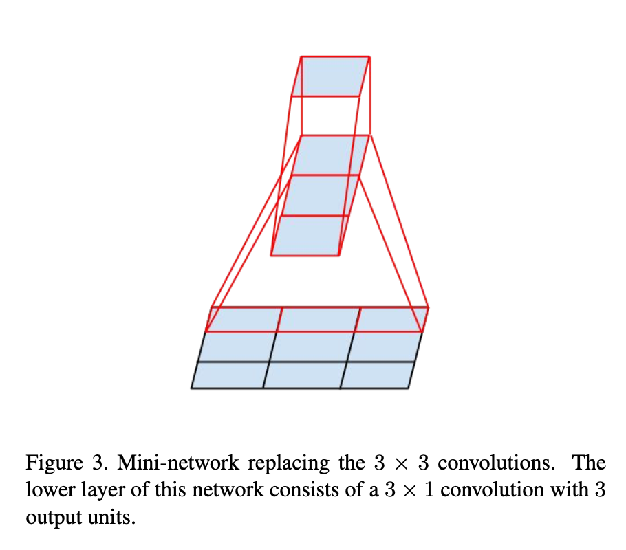
By using asymmetric convolutions, we can factorize 3 x 3 into smaller.

Using a 3 x 1 convolution followed by a 1 x 3 convolution is equivalent to sliding a two layer network with the same receptive field as in a 3 x 3 convolution.

We could go even further and argue that one can replace any $n$ x $n$ convolution by a 1 x $n$ convolution followed by $n$ x 1 convolution and the computational cost saving increases dramatically as $n$ grows.

→ Employing this factorization does not work well on early layers, but it gives very good results on medium grid sizes ( 12 < $n$ < 20 )

3×3 필터도 1×3 + 3×1로 나누면 추가적인 연산량 절감이 가능하다.

4. Utility of Auxiliary Classifiers

Most of paper argues that auxiliary classifiers promote more stable learning and better convergence.

Auxiliary Classifier
: 깊은 신경망에서 학습을 돕기 위해 중간 레이어에 추가되는 보조적인 분류기
→ 기울기 손실(vanishing gradient) 문제를 완화하고 학습을 촉진하는 역할

We found that auxiliary classifiers did not result in improved convergence early in the training.

1. Near the end of training, the network with the auxiliary branches starts to overtake the accuracy of the network without any auxiliary branch and reaches a slightly higher plateau.

( : auxiliary classifier가 accuracy에 효과를 미치는 때는 near the end of training이다. 그 전까지는 별 차이 없다. )

2. The removal of the lower auxiliary branch did not have any adverse effect on the final quality of the network.

1 + 2 → these branches help evolving the low-level features is most likely misplaced
Instead, we argure that the auxiliary classifiers act as regularizer.
→ This is supported by the main classifier of the network performs better if the side branch is batch-normalized or has a dropout layer

보조 분류기가 배치 정규화를 사용할 때 주 분류기의 성능이 향상된다.

결론적으로, auxiliary classifier(보조 분류기)가 정규화(regularization) 역할을 할 수 있다는 새로운 효율성을 발견한 것이다

5. Efficient Grid Size Reduction

Traditionally, convolutional networks used some pooling operation to decrease the grid size of the feature maps.

사용하던 전략
To avoid a representational bottleneck, before applying maximum or average pooling the activation dimension of the network filters is expanded.
: 네트워크가 충분한 정보를 유지한 상태에서 풀링을 수행하도록, 풀링 전에 활성화 차원을 늘려 representational bottleneck을 방지하는 전략

⬇️

문제점
This means that the overall computational cost is dominated by the expensive convolution on the larger grid.
: 활성화 차원을 확장하면 필터 개수가 늘어나므로, 이후 수행되는 합성곱 연산의 연산량이 증가함. 특히, 큰 크기의 특징 맵에서 합성곱을 수행하면 계산 비용이 급격히 상승할 수 있음

⬇️

해결책
One possibility would be to switch to pooling with convolution and therefore resulting in reducing the computational cost.
: 풀링을 합성곱과 함께 수행하는 것으로, 이를 통해 연산 비용을 줄일 수 있다

⬇️

또 다른 문제점
This creates a representational bottlenecks as the overall dimensionality of the representation drops, resulting in less expressive networks.
: 연산량을 줄일 수 있지만, 특징 맵의 크기가 빠르게 줄어들어 네트워크가 충분한 정보를 유지하지 못하는 representational bottleneck 현상이 발생한다..

그래서!
💁 : We suggest another variant the reduces the computational cost even further while removing the representational bottleneck. We can use two parallel stride 2 blocks : $P$(pool) and $C$(conv)

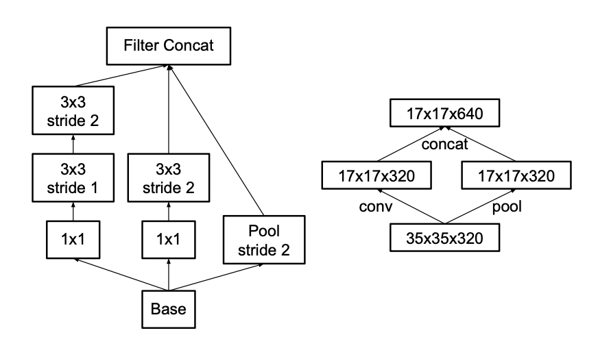
^ Inception module that reduces the grid-size while expands the filter banks. (Cheap & Avoids the representational bottleneck)

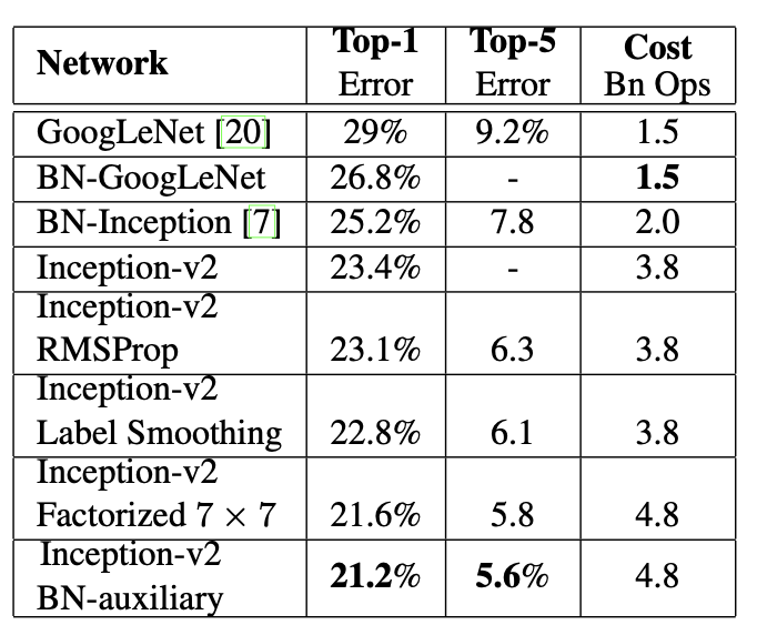
6. Inception-v2

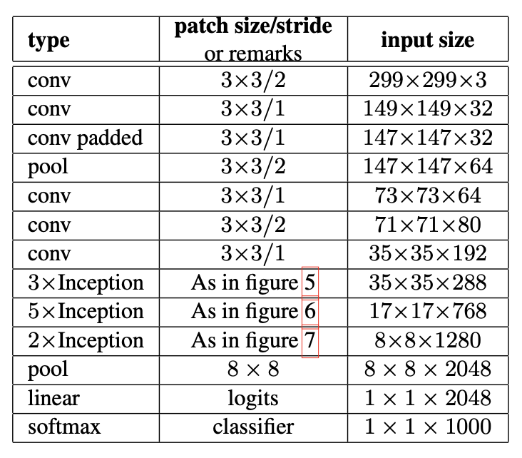
Layout of network
The output size of each module is the input size of the next one

Factorized the traditional 7 x 7 convolution into three 3 x 3 convolutions

💁 : We have observed that the quality of the network is relatively stable to variations as long as the principles from Section 2 are observed.

Section 2

• Avoid representational bottlenecks
• Higher dimensional representations
• Spatial aggregation
• Balance the width and depth of the network

7. Model Regularization via Label Smoothing

Regularize the classifier layer by estimating the marginalized effect of label-dropout during training.

label - dropout
: 일부 레이블을 제거(숨김)하여 모델이 부족한 라벨 데이터에서도 일반화할 수 있도록 학습하는 기법

For each training example $x$, our model computes the probability of each label

• $k ∈$ { $1 ... K$} : $p(k|x)$ = $exp(z_k) \over \sum_{i=1}^{K}exp(z_i)$
  • $z_i$ = logits or unnormalized log-probabilities

logit
: 로짓, 확률에 log(ln)을 취한 것

We define the loss as the cross entropy :

• $l$ = $- \sum_{k=1}^{K}log(p(k))q(k)$

Minimizing this is equivalent to maximizing the expected log-likelihood of a label, where the label is selected according to its ground-truth distribution $q(k)$.

Cross - entropy (H(p,q))
: 확률 분포 간 차이를 측정하는 손실 함수 (Loss Function)
→ 모델이 예측한 확률 분포와 실제 정답(라벨)의 분포 차이를 계산하여 손실(loss)로 변환

Cross-entropy loss is differentiable with respect to the logits $z_k$ and thus can be used for gradient training of deep models.

$q(y) = 1$ and $q(k) = 0$ for all $k≠y$.
In this case, Minimizing the cross entropy is equivalent to maximizing the log-likelihood of the correct label.
For particular example $x$ with label $y$, the log-likelihood is maximized for $q(k) = δ_{k,y}$

Dirac delta (δ(x))
: 특정 점에서만 무한한 값을 갖고, 나머지 구간에서는 0이 되는 함수
해당 점에서 적분하면 1이 되는 성질을 가지고 있다

If the logit corresponding to the groud-truth label is much great than all other logits.
However, it has 2 problems

• It may result in overfitting
  • it is not guaranteed to generalize
• It encourages the differences between the largest logit and all others to become large
  • with bounded gradient $∂l \over∂z_k$, reduces the ability of the model to adapt

This happens because the model becomes too confident about its predictions.

Encouraging the model to be less confident :
Consider a distribution over labels $u(k)$, independent of the training example $x$, and a smoothing parameter $ϵ$.

• $q(k|x) = δ_{k,y}$ → $q'(k|x) = (1-ϵ)δ_{k,y} + ϵu(k)$
  : mixture of the originial ground-truth distribution $q(k|x)$ and the fixed distribution $u(k)$, with weights $1 - ϵ$ and $ϵ$, respectively

We refer this change as label-smoothing regularization or LSR
LSR achieves the desired goal of preventing the largest logit from becoming much larger than all others.

Smoothing
: 데이터를 더 부드럽고 일반화된 형태로 변환하는 기법
→ 보통 급격한 변화 (Sharp Change)나 극단적인 값 (Extreme Value)을 완화하여, 더 일반적인 패턴을 학습하거나 표현하는 과정

Another interpretation of LSR can be obtained by considering the cross entropy ($H(q,p)$).
Thus, LSR is equivalent to replacing a single cross-entropy loss $H(q,p)$ with a pair of such losses $H(q,p)$ and $H(u,p)$.

The deviation $H(u,p)$ could be equivalently captured by the KL divergence, since $H(u,p) = D_{KL}(u||p) + H(u)$ and $H(u)$ is fixed.

KL divergence
: 두 확률분포 P(x)와 Q(x)가 얼마나 다른 지를 측정하는 비대칭적인 척도

• $D_{KL}(P||Q)$ = $\sum_x {P(x)\log{P(x)\over Q(x)}}$
  모델 Q가 진짜 분포 P를 얼마나 잘 설명했는가

8. Training Methodology

We have trained our networks with stochastic gradient utilizing the TenserFlow distributed machine learning system using 50 replicas running each on a NVidia Kepler GPU with batch size 32 for 100 epochs

9. Performance on Lower Resolution Input

A typical use-case of vision networks is for the post-classification of detection. The challenge is that objects tend to be relatively small and low-resolution.
→ how to properly deal with lower resolution input?
Common wisdom : employ higher resolution receptive fields

Need to distinguish between

• the effect of the increased resolution of the first layer receptive field → common wisdom
• the effects of larger model capacitance and computation

In order to make an accurate assessment, the model needs to analyze vague hints in oreder to be able to "hallucinate" the fine details.

hallucinate
→ 모델이 실제 데이터에는 없는 정보나 출력을 생성하는 것

how much does higher input resolution helps if the computational effort is kept constant?
→ Ensuring constant effort is to reduce the srides of the first two layer in the case of lower resolution input, or by simply removing the first pooling layer of the network.

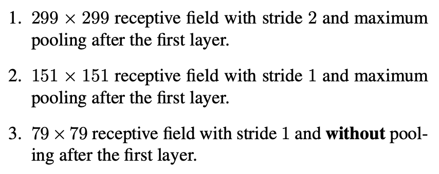
^ 3 experiments & results

If one would just naively reduce the network size according to the input resolution, then network would perform much more poorly.

10. Experimental Results and Comparisons

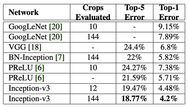
Inception-v3 → evalutae its performance in the multi-crop and ensemble settings

11. Conclusions

We have provided several design principles to scale up convolutional networks and studied them in the context of the Inception architecture.
This guidance can lead to high performance vision networks that have a relatively modest computation cost compared to simpler, more monolithic architectures.

We have also demonstrated that high quality results can be reached with receptive field resolution as low as 79 x 79.
→ helpful in systems for detecting relatively small objects

The combination of lower parameter count and additional regularization with batch-normalized auxiliary classifiers and label-smoothing allows for training high quality networks on relatively modest sized training sets.

끗!!