코드스테이츠 AI Bootcamp Section2에서 자유주제로 진행한 Machine Learning 개인프로젝트 내용 정리 및 회고. (1) 서론과 데이터준비 과정
- (1) 서론과 데이터준비 과정
- (2) 모델링 및 모델 하이퍼파라미터 튜닝
- (3) Model 해석, 결론, 회고
- Github Repository 바로가기 : Project-Hypertension-Predictive-Model (클릭)
한국형 고혈압 예측 모델 개발 (Hypertension Predictive Model)
- 고혈압 진단기준에 따른 차이가 있을까?

- Tech Stack

00. 프로젝트 개요
필수 포함 요소
자유 주제로 직접 선택한 데이터셋을 사용머신러닝 예측 모델을 통한성능 및 인사이트를 도출/공유- 데이터셋
전처리/EDA부터모델을 해석하는 과정까지 수행 - 발표를 듣는 사람은
비데이터 직군이라 가정
프로젝트 목차

-
Introduction
서론- Hypertension
고혈압 - Diagnotic Criteria
고혈압 진단기준 - Problems & Goals
문제정의 및 목표 - Dataset
선정 데이터셋 - Target & Features
타겟과 특성
- Hypertension
-
Data Preparation
데이터 준비- Data Pre-processing
데이터 전처리 - Final Data
최종데이터
- Data Pre-processing
-
Modeling
모델링- Data split
데이터 분리 - Baseline & Metrics
기준모델 및 평가지표 - Modeling(default)
기본값으로 모델링 - Hyperparameter Tuning
모델 튜닝 - Final Model & Test
최종모델 및 테스트
- Data split
-
Interpretation
해석- Feature Importance (MDI)
특성중요도 - Permutation Importance
순열중요도 - Feature Analysis (PDP)
특성 분석
- Feature Importance (MDI)
-
Conclusion
결론- Summary
요약 - Conclusion & Limitation
결론 및 한계점 - Retrospective
회고
- Summary
01. Introduction 서론
1-1. Hypertension 고혈압

- 고혈압 정의
- 동맥을 지나는 혈액의 압력이 지속적으로 정상기준보다 높아진 상태
침묵의 살인자
- 고혈압의 위험성
- 세계적으로 사망 위험요인 중 1위를 차지하는 만성질환
- 대표적 합병증
- 심혈관질환(뇌졸중,뇌출혈,심부전 등),고혈압성 망막증,신장기능저하 등...
- 고혈압 분류
- 본태성고혈압
뚜렷한 원인이 밝혀지지 않은 고혈압- 고혈압 환자의 95%가 이에 해당함
- 이차성고혈압
- 특정원인 질환에 의한 고혈압
- 수술 및 약물로 완치 가능
- 본태성고혈압
1-2. Diagnotic Criteria 고혈압 진단기준
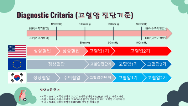
- 고혈압의 진단기준은 오랜기간 수축기혈압
140mmHg이상OR 이완기혈압90mmHg 이상이라는 진단 기준으로 진단되어 왔음. - 2017년, 미국 심장학회 및 심장협회에서 진단기준을 수축기혈압
130mmHg이상OR 이완기혈압80mmHg 이상으로 강화하였음. - 유럽과 대한민국의 경우엔 기존의 진단기준인 수축기혈압
140mmHg이상OR 이완기혈압90mmHg 이상을 유지하는 보수적인 입장을 취해오고 있음. - 현재까지도 어떤 진단기준을 따라야하는지에 대한 의견이 분분하여 지속적인 논의가 이루어지고 있는 상황임.
1-3. Problems & Goals 문제정의 및 목표
Problems 문제정의

고혈압 고위험군을 선별하고 고혈압을 예방하는 것은 중요한 문제- 고혈압 환자의 95%가 원인을 알 수 없는 본태성 고혈압
인공지능(AI) 머신러닝을 통한 예측 모델 개발 및 요인 분석의 필요성
각각의 진단기준에 따른 예측모델 개발 및 비교분석의 필요성
Goals 프로젝트 목표 및 가설
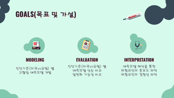
- 진단기준 별 고혈압 예측 모델 개발
- 진단기준 별 예측 모델의 성능 및 일반화가능성 비교분석
- 예측 모델 해석을 통한 위험요인의 중요도 및 경향성 파악
1-4. Dataset 선정 데이터셋

- 대한민국 질병관리청 국민건강영양조사 제8기 1,2차년도(2019~2020) 데이터셋
- 데이터셋 구성
- 검진조사, 건강설문조사, 영양조사
- 준비 과정
- 보안서약서 작성 후 SAS파일 다운로드
- SAS -> csv변환 -> 인코딩변환(utf-8) -> python으로 분석실시
1-5. Target & Features 타겟과 특성
Target 문제유형, 타겟
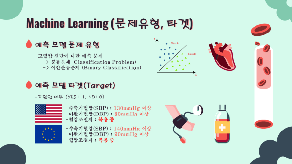
- 고혈압 진단 예측 모델이므로 이진분류문제(Binary Classification)로 정의
- 모델의 타겟은 고혈압 여부 (yes:1, no:0)
- 미국 진단기준 130mmHg↑ OR 80mmHg↑ OR 혈압조절제복용
- 유럽 진단기준 140mmHg↑ OR 90mmHg↑ OR 혈압조절제복용
Features 특성 선정

- 대한고혈압학회에서 정의한 위험요인 중에서 객관적인 수치화가 가능한 요인들을 선정하여 예측 모델의 특성으로 사용하였음.
02. Data Preparation 데이터 준비
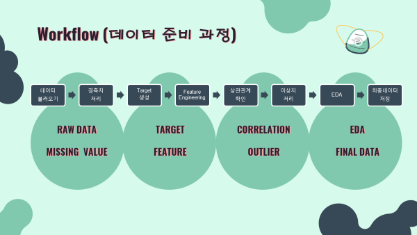
2-1. Data Pre-processing 데이터 전처리
STEP0. Library Import 라이브러리
import pandas as pd
# from pandas_profiling import ProfileReport
import numpy as np
import scipy as sp
import matplotlib.pyplot as plt
plt.rcParams['font.family'] = 'Malgun Gothic'
plt.rcParams['axes.unicode_minus'] = False
import seaborn as sns- 프로젝트 진행시 데이터를 파악하기 위해 pandas_profiling을 이용하였으나, 깃허브 페이지 표시오류가 발생하여 비활성화 시켰음.
STEP1. Data Import 데이터 불러오기
raw_2019 = pd.read_csv('data/2019_utf8.csv')
raw_2019.shape
#output
'''
(8110, 831)
'''
raw_2020 = pd.read_csv('data/2020_utf8.csv')
raw_2020.shape
#output
'''
(7359, 762)
'''STEP2. Feature & Target 정의, 추출, 병합
- 정의
demo_list = ['ID',
             'year',
             'sex',
             'age']
ques_list = ['DI1_2',
             'DI2_2',
             'DE1_31',
             'DE1_32',
             'DE1_dg',
             'BD1_11',
             'BD2_1',
             'sm_presnt']
exam_list = ['HE_HPfh1',
             'HE_HPfh2',
             'HE_sbp',
             'HE_dbp',
             'HE_wt',
             'HE_wc',
             'HE_BMI',
             'HE_glu',
             'HE_HbA1c',
             'HE_chol',
             'HE_TG']
column_list = demo_list+ques_list+exam_list- 추출
raw2_2019 = raw_2019[column_list]
raw2_2020 = raw_2020[column_list]
print(raw2_2019.shape)
print(raw2_2020.shape)
#output
'''
(8110, 23)
(7359, 23)
'''- 병합
raw_data = pd.concat([raw2_2019,raw2_2020],ignore_index=True)
raw_data.shape
#output
'''
(15469, 23)
'''
STEP3. 결측치 제거
- 결측치가
.으로 표기되어있어np.nan값으로 변환하였음.
#함수정의
def fillnan(value):
    if value == '.':
        value = np.nan
    return value
#함수적용
nanfill = raw_data.copy()
filled = nanfill.applymap(fillnan)
#확인
filled.info()
#output
'''
RangeIndex: 15469 entries, 0 to 15468
Data columns (total 23 columns):
 #   Column     Non-Null Count  Dtype
---  ------     --------------  -----
 0   ID         15469 non-null  object
 1   year       15469 non-null  int64
 2   sex        15469 non-null  int64
 3   age        15469 non-null  int64
 4   DI1_2      14802 non-null  object
 5   DI2_2      14802 non-null  object
 6   DE1_31     14802 non-null  object
 7   DE1_32     14802 non-null  object
 8   DE1_dg     14802 non-null  object
 9   BD1_11     14802 non-null  object
 10  BD2_1      14802 non-null  object
 11  sm_presnt  12048 non-null  object
 12  HE_HPfh1   13409 non-null  object
 13  HE_HPfh2   13409 non-null  object
 14  HE_sbp     13479 non-null  object
 15  HE_dbp     13479 non-null  object
 16  HE_wt      14760 non-null  object
 17  HE_wc      14073 non-null  object
 18  HE_BMI     14659 non-null  object
 19  HE_glu     13101 non-null  object
 20  HE_HbA1c   13097 non-null  object
 21  HE_chol    13101 non-null  object
 22  HE_TG      13101 non-null  object
dtypes: int64(3), object(20)
memory usage: 2.7+ MB
'''- ID를 제외한 모든 column 숫자형으로 변환
#숫자형 변환함수 적용
fix1 = filled.copy()
fix1.iloc[:,1:] = fix1.iloc[:,1:].apply(pd.to_numeric)
fix1.info()
#output
'''
RangeIndex: 15469 entries, 0 to 15468
Data columns (total 23 columns):
 #   Column     Non-Null Count  Dtype
---  ------     --------------  -----
 0   ID         15469 non-null  object
 1   year       15469 non-null  int64
 2   sex        15469 non-null  int64
 3   age        15469 non-null  int64
 4   DI1_2      14802 non-null  float64
 5   DI2_2      14802 non-null  float64
 6   DE1_31     14802 non-null  float64
 7   DE1_32     14802 non-null  float64
 8   DE1_dg     14802 non-null  float64
 9   BD1_11     14802 non-null  float64
 10  BD2_1      14802 non-null  float64
 11  sm_presnt  12048 non-null  float64
 12  HE_HPfh1   13409 non-null  float64
 13  HE_HPfh2   13409 non-null  float64
 14  HE_sbp     13479 non-null  float64
 15  HE_dbp     13479 non-null  float64
 16  HE_wt      14760 non-null  float64
 17  HE_wc      14073 non-null  float64
 18  HE_BMI     14659 non-null  float64
 19  HE_glu     13101 non-null  float64
 20  HE_HbA1c   13097 non-null  float64
 21  HE_chol    13101 non-null  float64
 22  HE_TG      13101 non-null  float64
dtypes: float64(19), int64(3), object(1)
memory usage: 2.7+ MB
'''- 결측치 포함된 row 제거
#drop
fix2 = fix1.copy()
fix2 = fix2.dropna().reset_index(drop=True)
fix2.info()
#output
'''
RangeIndex: 11573 entries, 0 to 11572
Data columns (total 23 columns):
 #   Column     Non-Null Count  Dtype
---  ------     --------------  -----
 0   ID         11573 non-null  object
 1   year       11573 non-null  int64
 2   sex        11573 non-null  int64
 3   age        11573 non-null  int64
 4   DI1_2      11573 non-null  float64
 5   DI2_2      11573 non-null  float64
 6   DE1_31     11573 non-null  float64
 7   DE1_32     11573 non-null  float64
 8   DE1_dg     11573 non-null  float64
 9   BD1_11     11573 non-null  float64
 10  BD2_1      11573 non-null  float64
 11  sm_presnt  11573 non-null  float64
 12  HE_HPfh1   11573 non-null  float64
 13  HE_HPfh2   11573 non-null  float64
 14  HE_sbp     11573 non-null  float64
 15  HE_dbp     11573 non-null  float64
 16  HE_wt      11573 non-null  float64
 17  HE_wc      11573 non-null  float64
 18  HE_BMI     11573 non-null  float64
 19  HE_glu     11573 non-null  float64
 20  HE_HbA1c   11573 non-null  float64
 21  HE_chol    11573 non-null  float64
 22  HE_TG      11573 non-null  float64
dtypes: float64(19), int64(3), object(1)
memory usage: 2.0+ MB
'''
STEP4. Target Data 생성
- Target Data 생성에 쓰일 column 추출
target_list = ['DI1_2','HE_sbp','HE_dbp']
target_df = fix2[target_list]
target_df.head()
- 혈압조절제 복용여부 column 생성
- 복용여부 : 설문지에 1,2,3,4 로 응답한 경우
#함수정의
bp_drug = []
for i in fix2.DI1_2:
    if i < 5:
        bp_drug.append(1)
    else:
        bp_drug.append(0)
bp_drug = np.array(bp_drug)
#적용
target_df2 = target_df.copy()
target_df2['bp_drug'] = bp_drug
target_df2.head()
- 미국 진단기준에 따른 고혈압 여부 column 생성
- 미국 진단기준 : 130mmHg↑ OR 80mmHg↑ OR 혈압조절제복용
#함수정의
hbp_us = []
for i in range(len(target_df2)):
    if (target_df2.loc[i,'HE_sbp']<130) & (target_df2.loc[i,'HE_dbp']<80) & (target_df2.loc[i,'bp_drug']==0):
        hbp_us.append(0)
    else:
        hbp_us.append(1)
hbp_us = np.array(hbp_us)
#적용
target_df3 = target_df2.copy()
target_df3['HBP_US'] = hbp_us
target_df3.head()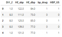
- 유럽 진단기준에 따른 고혈압 여부 column 생성
- 유럽 진단기준 : 140mmHg↑ OR 90mmHg↑ OR 혈압조절제복용
#함수정의
hbp_eu = []
for i in range(len(target_df2)):
    if (target_df2.loc[i,'HE_sbp']<140) & (target_df2.loc[i,'HE_dbp']<90) & (target_df2.loc[i,'bp_drug']==0):
        hbp_eu.append(0)
    else:
        hbp_eu.append(1)
hbp_eu = np.array(hbp_eu)
#적용
target_df4 = target_df3.copy()
target_df4['HBP_EU'] = hbp_eu
target_df4.head()
- 진단기준에따른 분포 시각화 (sklearn, matplotlib, seaborn)
#confusion metrix
from sklearn.metrics import confusion_matrix
cfm = confusion_matrix(target_df4.HBP_US,target_df4.HBP_EU)
#그룹명, 빈도, 백분율값
group_names = ['정상','-','당뇨병 전단계','당뇨병']
group_counts = ['{0:0.0f}'.format(value) for value in cfm.flatten()]
group_percentages = ['{0:.2%}'.format(value) for value in cfm.flatten()/np.sum(cfm)]
#label로 묶기, 축 label 설정
labels = [f'{v1}\n\n{v2}\n\n{v3}' for v1,v2,v3 in zip(group_names,group_counts,group_percentages)]
labels = np.asarray(labels).reshape(2,2)
tick = ['정상','고혈압']
#Heatmap 그리기
sns.heatmap(cfm, annot=labels, fmt='',cmap='Purples',xticklabels=tick,yticklabels=tick)
plt.xlabel('EU criteria')
plt.ylabel('US criteria')
plt.title('진단기준에 따른 분포\n[US : 130mmHg/80mmHg]\n[EU : 140mmHg/90mmHg]')
plt.show()
STEP5. Feature Engineering 특성가공
- Target에 이용한 column제외한 DataFrame 지정
feature_df = fix2.drop(columns=target_list,axis=1)
feature_df.shape
#output
'''
(11573, 20)
'''- 기본 정보(ID, 연도, 성별, 나이) column 추출
- 여기서 변수 하나씩 추가해서 DataFrame 구성할 예정
feature_df0 = feature_df[demo_list]
feature_df0.columns = ['ID','year','sex','age']
feature_df0.sample(5,random_state=42)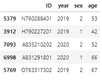
- 폭음여부 column 생성 및 추가
#list 생성
heavy_drink = []
for i in range(len(feature_df)):
    if (feature_df.loc[i,'sex']==1) & (feature_df.loc[i,'BD1_11'] in [3,4,5,6]) & (feature_df.loc[i,'BD2_1'] in [4,5]):
        heavy_drink.append(1)
    elif (feature_df.loc[i,'sex']==2) & (feature_df.loc[i,'BD1_11'] in [3,4,5,6]) & (feature_df.loc[i,'BD2_1'] in [3,4,5]):
        heavy_drink.append(1)
    else:
        heavy_drink.append(0)
heavy_drink = np.array(heavy_drink)
#column 추가
feature_df1 = feature_df0.copy()
feature_df1['heavy_drink'] = heavy_drink
feature_df1.sample(5,random_state=42)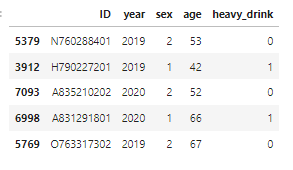
- 현재흡연여부 column 추가
#column 추가
feature_df2 = feature_df1.copy()
feature_df2['smoke'] = feature_df['sm_presnt'].astype(int)
feature_df2.sample(5,random_state=42)
- 가족력 column 생성 및 추가
- 1 : 가족력 없음 (혹은 미응답)
- 1.5 : 부모중 한쪽이 고혈압 진단
- 2 : 양쪽 부모 모두 고혈압 진단
- 한쪽 가족력 있을시 40~45%, 양쪽 가족력 있을시 80~90% 발병 위험이 높다는 근거에 의해 산출한 수치
#list 생성
genetic = []
for i in range(len(feature_df)):
    if (feature_df.loc[i,'HE_HPfh1']==1) & (feature_df.loc[i,'HE_HPfh2']==1):
        genetic.append(2)
    elif (feature_df.loc[i,'HE_HPfh1']==1) & (feature_df.loc[i,'HE_HPfh2']!=1):
        genetic.append(1.5)
    elif (feature_df.loc[i,'HE_HPfh1']!=1) & (feature_df.loc[i,'HE_HPfh2']==1):
        genetic.append(1.5)
    else:
        genetic.append(1)
genetic = np.array(genetic)
#column 추가
feature_df3 = feature_df2.copy()
feature_df3['genetic_hbp'] = genetic
feature_df3.sample(5,random_state=42)
- 체중, 허리둘레, BMI column 추가
#column 추가
exam_list0 = ['HE_wt','HE_wc','HE_BMI']
exam_list1 = ['weight','waist','BMI']
feature_df4 = feature_df3.copy()
feature_df4[exam_list1] = feature_df[exam_list0].astype(float)
feature_df4.sample(5,random_state=42)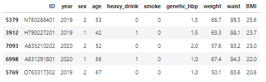
- 당뇨병여부 column 생성 및 추가
- 당뇨병 진단 기준 : 인슐린주사 OR 당뇨병약 OR 당뇨의사진단 OR 공복혈당 126이상 OR 당화혈색소 6.5이상
#list 생성
diabetes = []
for i in range(len(feature_df)):
    if (feature_df.loc[i,'DE1_31']!=1) & (feature_df.loc[i,'DE1_32']!=1) & (feature_df.loc[i,'DE1_dg']!=1) & (feature_df.loc[i,'HE_glu']<126) & (feature_df.loc[i,'HE_HbA1c']<6.5):
        diabetes.append(0)
    else:
        diabetes.append(1)
diabetes = np.array(diabetes)
#column 추가
feature_df5 = feature_df4.copy()
feature_df5['diabetes'] = diabetes
feature_df5.sample(5,random_state=42)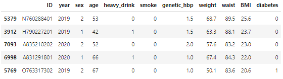
- 이상지질혈증(고콜레스테롤혈증) 여부 column 생성 및 추가
- 고콜레스테롤혈증 : 콜레스테롤조절제 OR 총콜레스테롤 수치 240상
#list 생성
hyper_chol = []
for i in range(len(feature_df)):
    if (feature_df.loc[i,'DI2_2'] > 4) & (feature_df.loc[i,'HE_chol'] < 240):
        hyper_chol.append(0)
    else:
        hyper_chol.append(1)
hyper_chol = np.array(hyper_chol)
#column 추가
feature_df6 = feature_df5.copy()
feature_df6['hyper_chol'] = hyper_chol
feature_df6.sample(5,random_state=42)
- 중성지방 column 추가
#column 추가
feature_df7 = feature_df6.copy()
feature_df7['triglycerides'] = feature_df['HE_TG'].astype(float)
feature_df7.sample(5,random_state=42)
- Target column 추가해서 마무리
#column 추가
fix_data0 = feature_df7.copy()
fix_data0[['HBP_US','HBP_EU']] = target_df4[['HBP_US','HBP_EU']]
fix_data0.info()
#output
'''
RangeIndex: 11573 entries, 0 to 11572
Data columns (total 15 columns):
 #   Column         Non-Null Count  Dtype
---  ------         --------------  -----
 0   ID             11573 non-null  object
 1   year           11573 non-null  int64
 2   sex            11573 non-null  int64
 3   age            11573 non-null  int64
 4   heavy_drink    11573 non-null  int32
 5   smoke          11573 non-null  int32
 6   genetic_hbp    11573 non-null  float64
 7   weight         11573 non-null  float64
 8   waist          11573 non-null  float64
 9   BMI            11573 non-null  float64
 10  diabetes       11573 non-null  int32
 11  hyper_chol     11573 non-null  int32
 12  triglycerides  11573 non-null  float64
 13  HBP_US         11573 non-null  int32
 14  HBP_EU         11573 non-null  int32
dtypes: float64(5), int32(6), int64(3), object(1)
memory usage: 1.1+ MB
'''
STEP6. 상관관계확인 & 다중공선성(노이즈 제거)
- 특성 & 타겟 상관관계 확인
- Data Leakage 방지
- 문제 없다 판단하고 진행하였음.
corr0 = fix_data0.corr(method='pearson')
corr0.iloc[1:,-2:].style.background_gradient(cmap='coolwarm',vmin=-1,vmax=1)
- 특성간 상관관계 확인(다중공선성)
check_features0 = fix_data0.iloc[:,2:-2]
feat_corr0 = check_features0.corr(method='pearson')
feat_corr0.style.background_gradient(cmap='coolwarm',vmin=-1,vmax=1)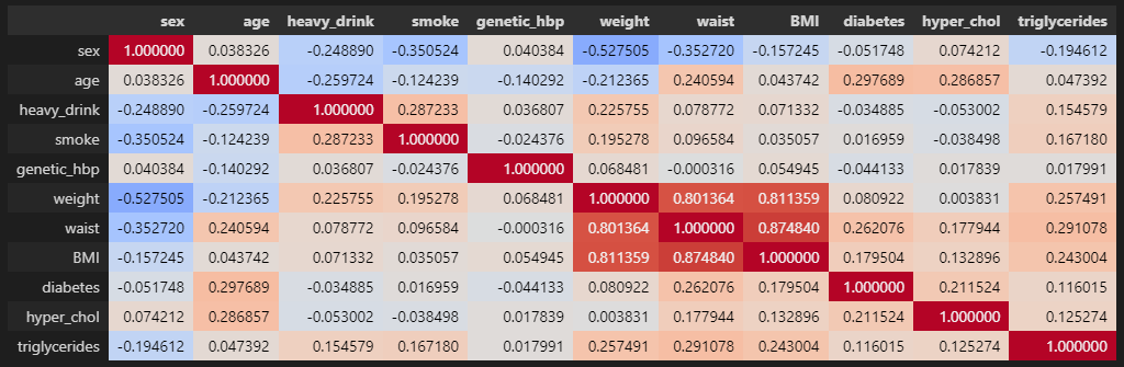
- 특성간 상관관계 시각화 (matplotlib, seaborn)
plt.figure(figsize=(12,8))
sns.heatmap(feat_corr0.round(2),
            cmap='coolwarm',
            annot=True,
            linewidths=.5,
            vmin=-1,
            vmax=1)
plt.show()
- 특성(독립변수)간의 강한 상관관계를 보이는 특성을 제거해 다중공선성 문제를 해결
- 강한 상관관계 특성 : 체중, 허리둘레, BMI
- 제거 특성 : 체중, 허리둘레
drop_list = ['weight','waist']
fix_data = fix_data0.copy()
fix_data = fix_data.drop(columns=drop_list,axis=1)
fix_data.info()
#output
'''
RangeIndex: 11573 entries, 0 to 11572
Data columns (total 13 columns):
 #   Column         Non-Null Count  Dtype
---  ------         --------------  -----
 0   ID             11573 non-null  object
 1   year           11573 non-null  int64
 2   sex            11573 non-null  int64
 3   age            11573 non-null  int64
 4   heavy_drink    11573 non-null  int32
 5   smoke          11573 non-null  int32
 6   genetic_hbp    11573 non-null  float64
 7   BMI            11573 non-null  float64
 8   diabetes       11573 non-null  int32
 9   hyper_chol     11573 non-null  int32
 10  triglycerides  11573 non-null  float64
 11  HBP_US         11573 non-null  int32
 12  HBP_EU         11573 non-null  int32
dtypes: float64(3), int32(6), int64(3), object(1)
memory usage: 904.3+ KB
'''- 제거후 특성 상관관계 시각화 (matplotlib, seaborn)
plt.figure(figsize=(12,8))
sns.heatmap(corr.round(2),
            cmap='coolwarm',
            annot=True,
            linewidths=.5,
            vmin=-1,
            vmax=1)
plt.show()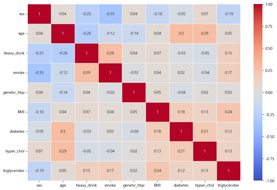
STEP7. 이상치 제거(노이즈 제거)
- 중성지방과 체질량지수(BMI) 데이터 분포상 이상치를 정의하고 제거하였음.
- 중성지방 : 500mg/dL 이상
- BMI : 40 이상
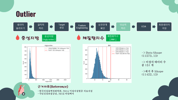
- 중성지방 분포 시각화 (matplotlib, seaborn)
sns.histplot(x='triglycerides',data=fix_data)
plt.axvline(200,label='고중성지방혈증 기준 (200mg/dL 이상)',linestyle='--',color='red',alpha=0.5)
plt.axvline(500,label='이상치 기준 (500mg/dL 이상)',linestyle='-',color='red',alpha=1)
plt.legend()
plt.title('triglycerides')
plt.show()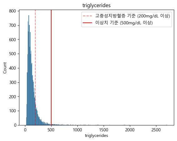
- BMI 분포 시각화 (matplotlib, seaborn)
sns.histplot(x='BMI',data=fix_data)
plt.axvline(25,label='1단계 비만(BMI 25 이상)',linestyle='--',color='red',alpha=0.4)
plt.axvline(30,label='2단계 비만(BMI 30 이상)',linestyle='--',color='red',alpha=0.6)
plt.axvline(35,label='3단계 비만(BMI 35 이상)',linestyle='--',color='red',alpha=0.8)
plt.axvline(40,label='이상치 기준 (BMI 40 이상)',linestyle='-',color='red',alpha=1)
plt.legend()
plt.title('BMI')
plt.show()
- 이상치 제거
#이상치 쿼리
outlier_BMI = fix_data.query('BMI >= 40')
outlier_chol = fix_data1.query('triglycerides >= 500')
# drop
fix_data1 = fix_data.drop(index=outlier_BMI.index).reset_index(drop=True)
fix_data2 = fix_data1.drop(index=outlier_chol.index).reset_index(drop=True)
#shape 변화확인
fix_data.shape
fix_data2.shape
#output
'''
(11573, 13)
(11422, 13)
'''
2-2. Final Data 최종데이터
최종 데이터 특성 EDA (탐색적분석)
- 최종데이터 정의 및 info
final_data = fix_data2.copy()
final_data.info()
#output
'''
RangeIndex: 11422 entries, 0 to 11421
Data columns (total 13 columns):
 #   Column         Non-Null Count  Dtype
---  ------         --------------  -----
 0   ID             11422 non-null  object
 1   year           11422 non-null  int64
 2   sex            11422 non-null  int64
 3   age            11422 non-null  int64
 4   heavy_drink    11422 non-null  int32
 5   smoke          11422 non-null  int32
 6   genetic_hbp    11422 non-null  float64
 7   BMI            11422 non-null  float64
 8   diabetes       11422 non-null  int32
 9   hyper_chol     11422 non-null  int32
 10  triglycerides  11422 non-null  float64
 11  HBP_US         11422 non-null  int32
 12  HBP_EU         11422 non-null  int32
dtypes: float64(3), int32(6), int64(3), object(1)
memory usage: 892.5+ KB
'''- 범주형 변수 barplot (matplotlib seaborn)
- 결과를 모아놓은 ppt 슬라이드로 출력을 대신하겠음
cat_cols = ['sex','heavy_drink','smoke','genetic_hbp','diabetes','hyper_chol']
for i in cat_cols:
    ax = sns.countplot(x=i,data=final_data)
    ax.bar_label(ax.containers[0])
    plt.title(i)
    plt.show()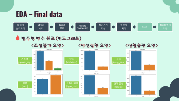
- 연속형 변수 histogram (matplotlib seaborn)
- 결과를 모아놓은 ppt 슬라이드로 출력을 대신하겠음
num_cols = ['age','BMI','triglycerides']
for i in num_cols:
    sns.histplot(x=i,data=final_data)
    plt.title(i)
    plt.show()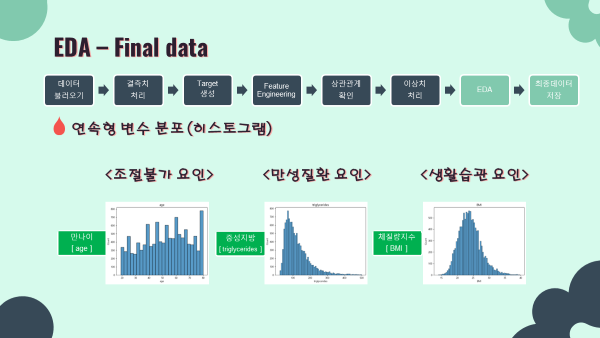
- 특성 상관관계 시각화 (matplotlib seaborn)
#feature 데이터 정의, 상관관계 DataFrame 생성
final_feature = final_data.drop(["ID","year","HBP_US","HBP_EU"],axis=1)
corr_final = final_feature.corr(method='pearson')
#plotting
fig, ax = plt.subplots(figsize=(12,8))
mask = np.zeros_like(corr_final,dtype=bool)
mask[np.triu_indices_from(mask)] = True
sns.heatmap(corr_final,
            cmap='coolwarm',
            annot=True,
            mask=mask,
            linewidths=.5,
            cbar_kws={'shrink':.5},
            vmin=-1,
            vmax=1)
plt.show()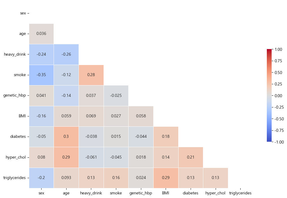
타겟 분포 확인
-
불균형은 없다 판단되어 이후 모델링에선 따로 전처리과정을 진행하지 않아도 될 것이라 판단함.
-
진단기준에 따른 분포 (sklearn matplotlib seaborn)
#confusion matrix
cfm_final = confusion_matrix(final_data.HBP_US,final_data.HBP_EU)
#표시할 값들 지정
group_names = ['정상','-','당뇨병 전단계','당뇨병']
group_counts = ['{0:0.0f}'.format(value) for value in cfm_final.flatten()]
group_percentages = ['{0:.2%}'.format(value) for value in cfm_final.flatten()/np.sum(cfm_final)]
labels = [f'{v1}\n\n{v2}\n\n{v3}' for v1,v2,v3 in zip(group_names,group_counts,group_percentages)]
labels = np.asarray(labels).reshape(2,2)
tick = ['정상','고혈압']
#히트맵 plot
sns.heatmap(cfm_final, annot=labels, fmt='',cmap='Purples',xticklabels=tick,yticklabels=tick)
plt.xlabel('EU criteria')
plt.ylabel('US criteria')
plt.title('진단기준에 따른 분포\n[US : 130mmHg/80mmHg]\n[EU : 140mmHg/90mmHg]')
plt.show()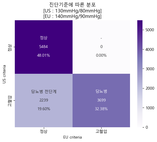
- 미국진단기준 고혈압 pie chart (matplotlib)
count_us = final_data.HBP_US.value_counts().sort_index()
count_label = ['정상(0)','고혈압(1)']
plt.pie(x = count_us,labels=count_label,autopct='%.2f%%',startangle=90)
plt.legend(loc = 'upper right')
plt.title('고혈압 비율\n[US criteria]')
plt.show()
- 유럽진단기준 고혈압 pie chart (matplotlib)
count_eu = final_data.HBP_EU.value_counts().sort_index()
count_label = ['정상(0)','고혈압(1)']
plt.pie(x = count_eu,labels=count_label,autopct='%.2f%%',startangle=90)
plt.legend(loc = 'upper right')
plt.title('고혈압 비율\n[EU criteria]')
plt.show()
최종 데이터 저장
final_data.to_csv('data/KNHANES_8th_final2.csv',index=False)03~. 이후 과정은 다음 포스팅에서!
- 내용이 너무 길어지는 관계로 이후 모델링 과정은 다음 포스팅에서 이어서 다루도록 하겠음.

일 때문에 포스팅은 잠시 쉬어요 ㅠ 바쁘다 바빠 모두들 화이팅! // Machine Learning (AI) Engineer & BackEnd Engineer (Entry)