Statistics 110 - Lecture 8

1. Binomial Distribution

    Binomial Distribution은 success의 확률에 대한 distribution이다. 아래와 같이 표현한다.

$X \sim Bin(n,p)$

• $n$ : 양의 정수 , $p$ : probability ( $0 \leq p \leq 1$)

강의에서 교수님이 Binomial distribution을 설명하실 때 3가지로 해석하신다. 하나씩 살펴보자.

1) Story

• $X$ : number of successes in $n$ independent $Bern(p)$ trials.
• $p$ : probability of success

→ Every trial results in success or failure, but not both.

2) Sum of Indicator Random Variables

• $X = X_1 + X_2 + \dots + X_n$
• $X_1, \dots ,X_n : i.i.d \ Bern(p)$, (i.i.d = independent, identically distributed )
  • = $X_1, \dots X_n$ have the same distribution.
• $X_j$ = 1 if jth trial = success, $X_j$ =0 otherwise

→ Indicator variable $X_j$ indicates whether the jth trial was a success or not.

→ exactly same as 1). (counting # of successes)

Random Variable VS Distribution

• distribution : explains how the probabilities of X will behave in different situations.
• multiple r.v.s can have the same distriution.

3) PMF (Probability Mass Function)

• def) probability of X on any particular value

  $P(X=k)= \binom{n}{k} \ p^k\ q^{n-k}, \ q=1-p$ (PMF for binomial dist.)

4) Binomial Distribution의 조건

• N identical trials.
• each trial being success or failure.
• probability of success must be same in all trials.
• each trial must be independent.

2. PMF (Probability Mass Function)

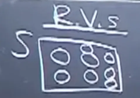
• S: sample space → different possible outcomes
• random variable : assigning a number to each pebble.
  • ex) $X=7$ is an event.
    • event = subset of sample space.
  • Can interpret this as a function.
    • Function that maps Sample space → interger (this case, 7)

1) CDF (Cumulative Distribution Function)

• $X \le x$ is an event.
• $F(x) = P(X \le x)$
  • $F$ : CDF of $X$.
• one way to describe a distribution.

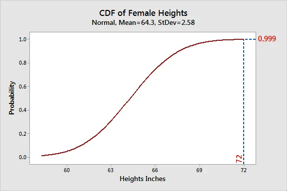
Continuous r.v.s' CDF

Discrete r.v.s' CDF

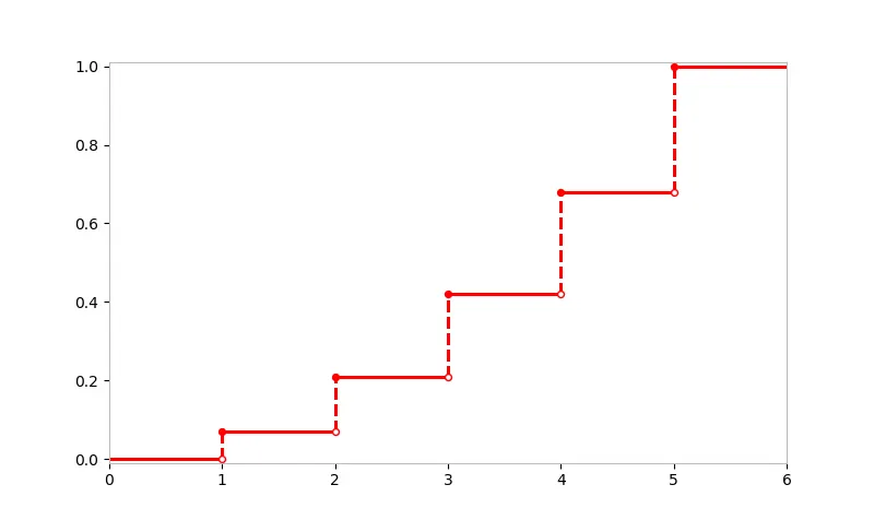
→ Good to have a visual idea of a CDF.

2) PMF - Discrete r.v.s

• Discrete r.v.s : possible values should be something you can list.
  • $a_1, a_2,\dots$ : could be infinite or finite
• PMF = $P(X=a_j)$ for all j.
  • 가능한 모든 값들에 대한 확률을 정의해야 함.
  • $p_j = P(X=a_j)$ 로 많이 표현함.
  • blueprint for X.
  • 조건 : $p_j \ge 0, \sum_j p_j =1$ (for discrete r.v.s)

Binomial Distribution PMF (revisit)

• $P(X=k)= \binom{n}{k} p^kq^{n-k}, \ q=1-p$ , $k \in \{0,1,\dots, n\}$
• 위의 조건 확인
  • $P(X=k) \ge 0$
  • sum : $\sum_{k=0}^n \binom nk p^kq^{n-k} = (p+q)^n =1^n = 1$, by Binomial Theorem.

Arithmetics between two distributions

• $X \sim Bin(n,p), Y \sim Bin(m,p)$, independent. Then, $X+Y \sim Bin(n+m,p)$
  • If the random variables are in the same sample space, you can add, subtract, multiply, divide.. etc. them.
  • Distributions should be Independent, probability of success must be same to use this property!

해석

1) Story

• adding two dist. is same as adding the number of successes from each trials.
  

2) Sum of Indicator Random Variables

• $X = X_1+\dots +X_n, Y=Y_1,\dots, Y_m$
• $X+Y = \sum_{j=1}^n X_j + \sum_{i=1}^m Y_i$
  → sum of $(n+m) \ \text{i.i.d}$ $\ Bern(p)$ = $Bin(n+m,p)$
  

3) PMF

• $P(X+Y=k) = \sum_{j=0}^k P(X+Y|X=j) \ P(X=j)$ (Law of total probability)
  $= \sum_{j=0}^k P(Y=k-j|X=j)\binom njp^jq^{n-j}$ ($P(X=j)$ → use PMF directly)

→ $X, Y$ are independent, so $P(Y=k-j|X=j) = P(Y=k-j)$ (X has no impact on Y.)

= $\sum_{j=0}^k \binom m {k-j} p^{k-j} \ q^{m-k+j}\binom njp^j\ q^{n-j}$
= $p^kq^{m+n-k} \ \sum_{j=0}^k \binom m {k-j} \binom n j = \binom {m+n} k$ (VanderMonde Identity)

-> so PMF proves that $X+Y \sim Bin(n+m,p)$ is TRUE.

3. Common Mistakes - Thinking that it is a Binomial when it’s not.

• Ex1) 5 card hand from a 52 card deck. → Find distribution of the number of aces in the hand. → PMF or CDF
  • Let $X = (\text{\# of aces})$
  • PMF
    • Find $P(X=k)$ , This is 0 except if $k \in \{0,1,2,3,4\}$
      • Distribution is NOT Binomial.
        • trials are not independent.
          • if one ace comes out, prob. of success changes in the next trial.
    • $P(X=k) = \frac{\binom 4 k \binom {48}{5-k}}{\binom {52}{5}}$ for $k \in \{0,1,2,3,4\}$
      • same as elk problem (from h.w.)
        • some elks are tagged, some are not. → when collecting a sample, what is the prob. of the collected sample has exactly k tagged elks?
• Ex) Have b black, and w white marbles , pick simple random samples(= all subsets of that size are equally likely)of size n.

→ Find the Distribution of # of white marbles in the sample (pretty much the same as ex1.)

• $P(X=k) = \frac{\binom w k \binom {b}{n-k}}{\binom {w+b}{n}}$ , $0 \le k \le w, 0 \le n-k \le b$
• This Distribution is called Hypergeometric distribution.
• sampling without replacement. (trials are not independent, so not binomial)
• If you sample with replacement, it will be Binomial!

Validation of the Hypergeometric Dist. PMF

$P(X=k) = \frac{\binom w k \binom {b}{n-k}}{\binom {w+b}{n}}$, $0 \le k \le w, 0 \le n-k \le b$

• Sum = 1?
  • $\sum_{k=0}^w \frac{\binom w k \binom {b}{n-k}}{\binom {w+b}{n}} = \frac {\sum_{k=0}^w \binom w k \binom {b}{n-k}}{ \binom {w+b}{n}} \ = 1$ (via VanderMonde)