cs231n 과제1 Q2- Training a SVM

  cs231n 과제 1 Q2를 하면서 내가 헷갈렸거나 몰랐던 것들을 정리해보려고 한다. 생각보다 꽤 어렵지만 풀었을때 기분이 좋긴 한 것 같다. 일단 A1을 최대한 빨리 끝내는 것이 중요할 것 같다.

1. svm_loss_naive 함수

  이 함수는 linear_svm.py에 있는 함수이다.

 for i in range(num_train):
        scores = X[i].dot(W)
        correct_class_score = scores[y[i]] #eqivalent to s_yi in slides
        for j in range(num_classes):
          margin = scores[j] - correct_class_score + 1 
          if j == y[i]: # if the correct class== the class we are paying attention
            continue
          if margin>0:
            loss+=margin
            dW[:,y[i]]-=X[i]
            dW[:,j]+=X[i]


    # Right now the loss is a sum over all training examples, but we want it
    # to be an average instead so we divide by num_train.
    loss /= num_train

    # Add regularization to the loss.
    loss += reg * np.sum(W * W) # L2 loss

    #############################################################################
    # TODO:                                                                     #
    # Compute the gradient of the loss function and store it dW.                #
    # Rather than first computing the loss and then computing the derivative,   #
    # it may be simpler to compute the derivative at the same time that the     #
    # loss is being computed. As a result you may need to modify some of the    #
    # code above to compute the gradient.                                       #
    #############################################################################
    # *****START OF YOUR CODE (DO NOT DELETE/MODIFY THIS LINE)*****
    dW/=num_train
    dW+=2*reg*W
   

  함수의 모든 부분을 가져온 것은 아니다. 여기서 내가 어려웠던 것은 margin>0인 경우에 $dW$를 계산하는 부분이다. 일단 svm function을 내가 미분해서, 코드에 맞게 변형해야 한다.

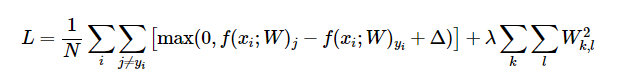
  기본적으로 위의 loss function을 바탕으로 미분을 진행한다. 이렇게 보면 어려워보이지만, 그 의미를 생각하면 할 수 있다.

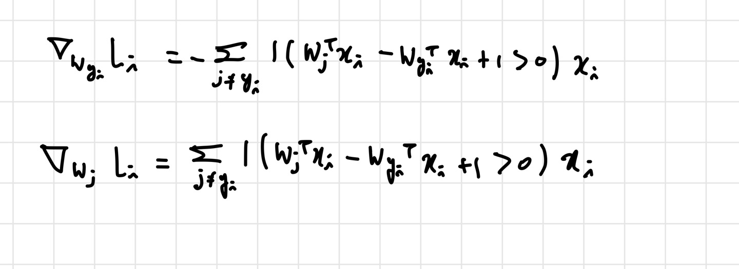
loss function에서 $y_i$와 $j$가 같은 경우는 제외하고 계산하기 때문에, $y_i$에 대해 미분한 것과 $j$에 대해 미분한 것을 구별해줘야 한다. 물론 위의 식에 regularization도 미분한 걸 적용해줘야 한다.

2. svm_loss_vectorized

correct_y_scores=scores[np.arange(num_train), y].reshape(num_train,1)
    margin=np.maximum(scores-correct_y_scores+1,0)
    margin[np.arange(num_train), y] = 0 # Correct class=0
    loss=np.sum(margin)/num_train
    loss += reg * np.sum(W * W)


    # *****END OF YOUR CODE (DO NOT DELETE/MODIFY THIS LINE)*****

    #############################################################################
    # TODO:                                                                     #
    # Implement a vectorized version of the gradient for the structured SVM     #
    # loss, storing the result in dW.                                           #
    #                                                                           #
    # Hint: Instead of computing the gradient from scratch, it may be easier    #
    # to reuse some of the intermediate values that you used to compute the     #
    # loss.                                                                     #
    #############################################################################
    # *****START OF YOUR CODE (DO NOT DELETE/MODIFY THIS LINE)*****
    dW=(margin>0).astype(int) #111...0111 -> correct class has label 0.
    dW[np.arange(num_train),y]-=dW.sum(axis=1)#dW has shape (3073,10)-> so sum w.r.t class dimension. we subtract (classes-1) -> 1 being correct class.
    dW=X.T.dot(dW)/num_train +2*reg*W

  이건 위의 naive 버전을 vectorize 한 함수이다. 마찬가지로 내가 헷갈렸던 부분만 가져왔다. 여기서 어려웠던 부분은 margin 행렬에서, $y_i$ != $j$인 자리에서는 margin을 제대로 계산하고 $y_i$==$j$인 class들 자리에는 0을 넣는다는 것이다. 이게 말로는 쉬운데, margin 값을 다 계산하고 그 이후에 margin[np.arange(num_train),y]로 접근할 생각을 못했다. np.arange(num_train)을 사용하면 모든 샘플의 참 클래스 자리로 접근할 수 있다.
이렇게 만들어놓은 상태에서 dW=(margin>0).astype(int) 를 하면, margin>0인 원소들은 모두 1이 된다. 그리고 y_i==j인 자리에는 -X[i]를 해주어야 하기 때문에 위에서
dW[np.arange(num_train),y]-=dW.sum(axis=1)를 해주는 것이다. 그리고 이렇게 업데이트 된 dW에 X를 곱해주면, 우리는 vectorized 된 version으로 코드를 완성할 수 있다.
이 파트에서 제일 떠올리기 어려웠던 아이디어는 X 행렬을 나중에 곱한다는 생각이다. 먼저 dW 행렬을 1과 0으로 무시할 원소와 값이 있는 원소들로 나눈 후, 마지막에 한 방에 X를 곱하는 것이 인상적이었다.

내 풀이 링크:

https://github.com/danlee0113/cs231n