cs231n 과제3 Q4- Self-Supervised Learning for Image Classification

  이번 주제는 내가 들은 cs231n 2017 버전 강의로는 접해보지 못했던 주제이다. 강의에서 구현하는 SimCLR 논문이 2020년에 나왔으니 그럴만 하다. 논문을 다 읽어본 것은 아니지만, 논문에서 사용하는 컨셉이 굉장히 참신하다. 이번 글에서는 Self-Supervised Learning이 무엇인지 대략적으로 정리하고, 내가 헷갈렸던 부분을 적어보려고 한다.

1. Self-Supervised Learning(SSL)

  기존의 ML method에는 labeled data를 이용하는 supervised learning이 많이 등장한다. 그러나 supervised learning은 dataset labeling을 사람이 해야 해서 아주 큰 데이터셋을 만들기는 힘들다. 그래서 등장한 개념이 Self-supervised learning이다. label된 데이터셋이 없이 모델을 훈련시켜 좋은 visual representation을 만들어내는 것이다. SSL이 많이 사용되는 이유는 모델이 훈련에 사용하지 않은 아예 새로운 dataset에 대해서도 좋은 성능을 내기 때문이다.
  SSL의 개념을 처음 들으면 드는 의문이 '좋은 representation이란 무엇인가?' 이다. 좋은 representation vector는 영상의 중요한 feature를 잡아내야 한다. 비슷한 영상들은 (semantically similar) 비슷한 representation vector를 가져야 하는 것이다. SimCLR 논문은 좋은 representation을 배우기 위해 contrastive learning이라는 방법을 사용한다. contrastive learning은 비슷한 영상은 비슷한 representation vector를 갖게 하는 것을 목표로 한다. 이를 위해 각 image에 대해 네트워크는 positive pair라고 불리는 2개의 이미지를 생성한다. 이때 2개의 이미지는 서로 다른 data augmentation 방법을 이용해 만들어진 이미지이다. 즉, 한 개의 input image당 2개의 data augemented image가 생기는 것이다.

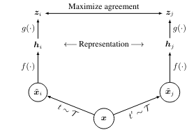
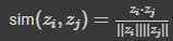
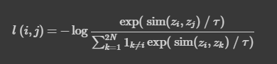
  이것이 모델에서 사용하는 contrastive learning의 구조도이다. $\tilde{x_i}$와 $\tilde{x_j}$는 위에서 언급한 data augmented image를 의미한다. $t$와 $t'$는 사용한 augmentation scheme에 해당한다. 이렇게 나온 두 개의 image는 기본적인 encoder net인 $f$에 먹여지고, $f$를 통해 우리는 representation vector $h_i,h_j$를 얻게 된다. 논문에서는 ResNet을 encoder network로 사용했다. 마지막으로, network projection head인 $g$를 거쳐 contrastive loss를 계산할 수 있는 $z_i,z_j$가 나오게 된다. 모델의 목표는 $z_i와 z_j$ 간의 agreement를 최대화 하는 것이다. 구체적인 loss는 아래와 같이 계산한다. $sim(z_i,z_j)$는 두 벡터의 dot product/(각 vector의 norm)을 의미하는데, 이렇게 식을 구성하면 우리가 앞서 이야기한 $z_i와 z_j$의 agreement를 높이는 일이 가능해진다. dot product는 두 벡터의 simliarity가 높을수록 커지기 때문이다. $\tau$ 값은 exp가 증가하는 속도를 조절해주는 값이다.

각 벡터에 대해 loss를 계산하는 방법

total loss를 계산하는 식

이제 코드를 보며 이 모델을 구현해보자.

2. Implementation

1) data augmentation

def compute_train_transform(seed=123456):
    """
    This function returns a composition of data augmentations to a single training image.
    Complete the following lines. Hint: look at available functions in torchvision.transforms
    """
    random.seed(seed)
    torch.random.manual_seed(seed)
    
    # Transformation that applies color jitter with brightness=0.4, contrast=0.4, saturation=0.4, and hue=0.1
    color_jitter = transforms.ColorJitter(0.4, 0.4, 0.4, 0.1)  
    
    train_transform = transforms.Compose([
        ##############################################################################
        # TODO: Start of your code.                                                  #
        #                                                                            #
        # Hint: Check out transformation functions defined in torchvision.transforms #
        # The first operation is filled out for you as an example.
        ##############################################################################
        # Step 1: Randomly resize and crop to 32x32.
        transforms.RandomResizedCrop(32),
        # Step 2: Horizontally flip the image with probability 0.5
        transforms.RandomHorizontalFlip(p=0.5),
        # Step 3: With a probability of 0.8, apply color jitter (you can use "color_jitter" defined above.
        transforms.RandomApply([color_jitter], p=0.8),
        # Step 4: With a probability of 0.2, convert the image to grayscale
        transforms.RandomGrayscale(p=0.2),
        ##############################################################################
        #                               END OF YOUR CODE                             #
        ##############################################################################
        transforms.ToTensor(),
        transforms.Normalize([0.4914, 0.4822, 0.4465], [0.2023, 0.1994, 0.2010])])
    return train_transform

  랜덤하게 data augmentation을 적용하는 과정이다. 각 augmentation method마다 확률 값을 주어서 랜덤성을 부여한 것을 볼 수 있다. 그리고 나서 loss를 계산하는 함수를 구현하는데, naive 버전은 for문을 사용하면 돼서 그닥 어렵지 않다.

def simclr_loss_vectorized(out_left, out_right, tau, device='cuda'):
    """Compute the contrastive loss L over a batch (vectorized version). No loops are allowed.
    
    Inputs and output are the same as in simclr_loss_naive.
    """
    N = out_left.shape[0]
    
    # Concatenate out_left and out_right into a 2*N x D tensor.
    out = torch.cat([out_left, out_right], dim=0)  # [2*N, D]
    
    # Compute similarity matrix between all pairs of augmented examples in the batch.
    sim_matrix = compute_sim_matrix(out)  # [2*N, 2*N]
    
    ##############################################################################
    # TODO: Start of your code. Follow the hints.                                #
    ##############################################################################
    
    # Step 1: Use sim_matrix to compute the denominator value for all augmented samples.
    # Hint: Compute e^{sim / tau} and store into exponential, which should have shape 2N x 2N.
    exponential = None
    exponential=torch.exp(sim_matrix/tau)
    # This binary mask zeros out terms where k=i.
    mask = (torch.ones_like(exponential, device=device) - torch.eye(2 * N, device=device)).to(device).bool()
    
    # We apply the binary mask.
    exponential = exponential.masked_select(mask).view(2 * N, -1)  # [2*N, 2*N-1]
    
    # Hint: Compute the denominator values for all augmented samples. This should be a 2N x 1 vector.
    denom = None

    # Step 2: Compute similarity between positive pairs.
    # You can do this in two ways: 
    # Option 1: Extract the corresponding indices from sim_matrix. 
    # Option 2: Use sim_positive_pairs().
    # *****START OF YOUR CODE (DO NOT DELETE/MODIFY THIS LINE)*****

    denom=exponential.sum(dim=1) #exponential is the index extracted version of sim_matrix.
    # *****END OF YOUR CODE (DO NOT DELETE/MODIFY THIS LINE)*****
    
    # Step 3: Compute the numerator value for all augmented samples.
    numerator = None
    # *****START OF YOUR CODE (DO NOT DELETE/MODIFY THIS LINE)*****

    n1=sim_matrix[torch.arange(N),torch.arange(N)+N]
    n2=sim_matrix[torch.arange(N)+N,torch.arange(N)]
    numerator=torch.cat([n1,n2],dim=0)
    numerator=torch.exp(numerator/tau)
    # *****END OF YOUR CODE (DO NOT DELETE/MODIFY THIS LINE)*****
    
    # Step 4: Now that you have the numerator and denominator for all augmented samples, compute the total loss.
    loss = None
    # *****START OF YOUR CODE (DO NOT DELETE/MODIFY THIS LINE)*****

    loss = -torch.log(numerator / denom)
    loss = torch.sum(loss)
    loss /= 2*N

    # *****END OF YOUR CODE (DO NOT DELETE/MODIFY THIS LINE)*****
    
    ##############################################################################
    #                               END OF YOUR CODE                             #
    ##############################################################################
    
    return loss

  위의 코드가 loss를 계산하는 vectorized 버전인데, 여기서 애를 좀 먹었다. vecotrized 코드로 loss 식을 바꿀때, k==i인 원소는 제외해야 하므로, mask를 씌워서 계산해주어야 한다. step 2에서 준 힌트는 sim_matrix를 이용하거나 sim_positive_pair 함수를 이용하라고 했다. 그래서 나는 sim_matrix에서 사용할 index를 빼내려고 노력했는데, 알고 보니 exponential이 sim_matrix에 mask를 씌워 index를 걸러낸 상태였기 때문에 그냥 exponential을 이용하면 되는 것이었다. (sim_matrix와 sim_positive 함수가 무엇인지는 전체 코드를 보면 알 수 있다.)

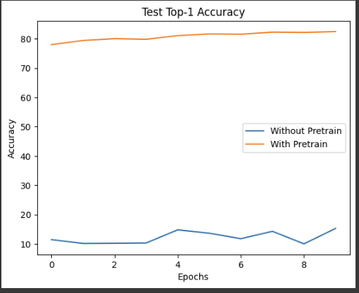
  이런 식으로 훈련하면 test top-1 accuracy가 엄청나게 차이나는 것을 볼 수 있다. label을 사용하지 않고도 이렇게 좋은 성능을 낼 수 있다는 것이 굉장히 신기했다. 또, 큰 데이터셋에서 모델을 훈련시켜야만 좋은 성능을 낼 수 있다는 고정관념을 어느 정도 깨 준 방식인 것 같다.

내 과제 풀이:

https://github.com/danlee0113/cs231n