Logistic Regression

필요성

다중선형회귀모델에서, 예측변수 y가 범주형 (예 / 아니오 , 1 / 0 , 참 / 거짓, 합격 / 불합격 ) 이라면 오류가 발생한다. 따라서 로지스틱 회귀모형이 필요 !

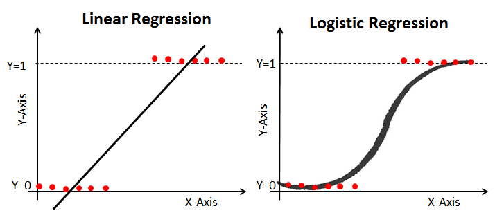
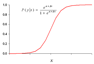
직선인 선형회귀로는 fitting이 어렵기 때문에 S자형 곡선인 로지스틱 함수를 이용한다. ( 로짓변환 )

---

Odds (승산)

• 오즈 : 임의의 이벤트가 발생하지 않을 확률 대 비 발생할 확률 (실패에 비해 성공할 확률의 비)
  $Odds = p / (1-p)$

• 오즈비(odds ratio) : 오즈 간의 비율
  

---

로짓변환

$logit = log(odds) = log(p / (1-p))$

‣ 일반선형 회귀모형 : $f(x) = b_0 + b_1X_1 + ... b_pX_p$
‣ 다중선형 회귀모형 : $y = b_0 + b_1X_1 + ... b_pX_p$
‣ 로지스틱 회귀모형 : $ln(p/1-p) = b_0 + b_1X_1 + ... b_pX_p$

⋙ 즉, 로지스틱 회귀분석은 일반회귀모형의 링크함수( $f(x)$) 를 로짓으로 변형한 분석이다.
.
.
.
▣ 독립변수가 1개인 상황의 로지스틱 회귀분석 식을 정리해보자.

$ln(p /(1-p)) = a +bX$
$p/(1-p) = e^{a+bX}$
$p = {e^{a+bX}}/(1+e^{a+bX})$ : 시그모이드 함수

---

Scikit-Learn 로지스틱 회귀분석

‣ data : Iris

‣ 4개의 feature들로 iris의 품종 ( 0,1,2 ) 을 분류하는 분류기 만들기.

import numpy as np
import pandas as pd
import matplotlib.pyplot as plt
import seaborn as sns

from sklearn.datasets import load_iris
from sklearn.model_selection import train_test_split  
from sklearn.linear_model import LogisticRegression
from sklearn.metrics import RocCurveDisplay, roc_auc_score
from sklearn.metrics import r2_score, mean_squared_error 

iris = load_iris()
print(iris.target_names)
# ['setosa' 'versicolor' 'virginica']

print(iris.feature_names)
# ['sepal length (cm)',
#  'sepal width (cm)',
#  'petal length (cm)',
#  'petal width (cm)']

X,y = load_iris(return_X_y = True)
print(X[:5], X.shape) 
# [[5.1 3.5 1.4 0.2]
#  [4.9 3.  1.4 0.2]
#  [4.7 3.2 1.3 0.2]
#  [4.6 3.1 1.5 0.2]
#  [5.  3.6 1.4 0.2]]

# (150, 4)

print(y, y.shape) 
# [0 0 0 0 0 0 0 0 0 0 0 0 0 0 0 0 0 0 0 0 0 0 0 0 0 0 0 0 0 0 0 0 0 0 0 0 0
#  0 0 0 0 0 0 0 0 0 0 0 0 0 1 1 1 1 1 1 1 1 1 1 1 1 1 1 1 1 1 1 1 1 1 1 1 1
#  1 1 1 1 1 1 1 1 1 1 1 1 1 1 1 1 1 1 1 1 1 1 1 1 1 1 2 2 2 2 2 2 2 2 2 2 2
#  2 2 2 2 2 2 2 2 2 2 2 2 2 2 2 2 2 2 2 2 2 2 2 2 2 2 2 2 2 2 2 2 2 2 2 2 2
#  2 2]

# (150, )

data split

X_train, X_test, y_train, y_test = train_test_split(X, y, stratify = y, random_state = 10)
print(X_train.shape, X_test.shape, y_train.shape, y_test.shape)
# (112, 4) (38, 4) (112,) (38,)

print(np.unique(y_test, return_counts = True))
# (array([0, 1, 2]), array([12, 13, 13], dtype=int64))
# 0,1,2 가 적절한 비율로 나눠진 것 확인 가능

모델 적합

• LogisticRegression

m = LogisticRegression(solver = 'liblinear')

• solver

  ▢ For small datasets, ‘liblinear’ is a good choice, whereas ‘sag’ and ‘saga’ are faster for large ones;
  ▢ For multiclass problems, only ‘newton-cg’, ‘sag’, ‘saga’ and ‘lbfgs’ handle multinomial loss;
  ▢ 'liblinear' is limited to one-versus-rest schemes.
  ▢ 'newton-cholesky' is a good choice for n_samples >> n_features, especially with one-hot encoded categorical features with rare categories. Note that it is limited to binary classification and the one-versus-rest reduction for multiclass classification. Be aware that the memory usage of this solver has a quadratic dependency on n_features because it explicitly computes the Hessian matrix.

m.fit(X_train, y_train)
pred = m.predict(X_test)
print(r2_score(y_test, pred))
# 0.9599578503688093