의사결정나무(Decision Tree)

의사결정나무란?

의사결정나무(Decision Tree)는 주어진 독립변수에 의사결정규칙을 적용해 나가면서 종속변수를 예측해 나가는 알고리즘이다. 분류와 회귀에 모두 사용할 수 있다. 종속변수에 따라 분류나무와 회귀나무로 구분된다.

의사결정규칙(가지분할)을 만들 때 기준이 될 독립변수 항목과 값을 선택하는 방법이 있다.

• 분류나무 : 카이제곱 통계량의 p값, 지니지수, 엔트로피지수
• 회귀나무 : F 통계량의 p값, 분산의 감소량

의사결정나무 알고리즘에는 CART, CHAID, ID3, C4.5, C5.0, MARS 등의 다양한 방법론이 존재한다. 이 중에서 CART 알고리즘을 이용해 실습한다.

Data Load

> train <- read.csv('ch6-2_train.csv', header=TRUE)
> test <- read.csv('ch6-2_test.csv', header=TRUE)

패키지 설치 및 불러오기

CART 수행을 위한 패키지이다.

> install.packages('rpart')
> library(rpart)

의사결정나무

rpart 패키지의 rpart() 함수를 이용해 의사결정나무를 수행한다. 만든 모델을 확인해보면 독립변수 항목과 값에 따라 의사결정 노드들이 만들어진 것을 확인할 수 있다. 하지만 텍스트로 되어있어 결과를 보기가 어렵다.

> dt <- rpart(breeds ~ ., data=train)
> dt
n= 240 

node), split, n, loss, yval, (yprob)
      * denotes terminal node

 1) root 240 160 a (0.33333333 0.33333333 0.33333333)  
   2) tail_length< 67.5 113  33 a (0.70796460 0.29203540 0.00000000)  
     4) wing_length>=231.5 82   4 a (0.95121951 0.04878049 0.00000000) *
     5) wing_length< 231.5 31   2 b (0.06451613 0.93548387 0.00000000) *
   3) tail_length>=67.5 127  47 c (0.00000000 0.37007874 0.62992126)  
     6) wing_length< 226.5 34   3 b (0.00000000 0.91176471 0.08823529) *
     7) wing_length>=226.5 93  16 c (0.00000000 0.17204301 0.82795699)  
      14) comb_height>=36.5 15   6 b (0.00000000 0.60000000 0.40000000) *
      15) comb_height< 36.5 78   7 c (0.00000000 0.08974359 0.91025641) *

의사결정나무 그래프

rpart.plot 패키지를 불러온 뒤 prp() 함수를 통해 트리 모양의 그래프를 그릴 수 있다.

> install.packages('rpart.plot')
> library(rpart.plot)

> prp(dt, type=4, extra=2, main='Decision Tree')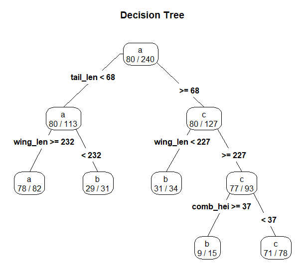

모델 성능 평가

> test$breeds <- as.factor(test$breeds)
> test$pred <- predict(dt, newdata=test, type="class")

> library(caret)
> confusionMatrix(test$pred, test$breeds)
Confusion Matrix and Statistics

          Reference
Prediction  a  b  c
         a 19  2  0
         b  1 16  4
         c  0  2 16

Overall Statistics
                                         
               Accuracy : 0.85           
                 95% CI : (0.7343, 0.929)
    No Information Rate : 0.3333         
    P-Value [Acc > NIR] : < 2.2e-16      
                                         
                  Kappa : 0.775          
                                         
 Mcnemar's Test P-Value : NA             

Statistics by Class:

                     Class: a Class: b Class: c
Sensitivity            0.9500   0.8000   0.8000
Specificity            0.9500   0.8750   0.9500
Pos Pred Value         0.9048   0.7619   0.8889
Neg Pred Value         0.9744   0.8974   0.9048
Prevalence             0.3333   0.3333   0.3333
Detection Rate         0.3167   0.2667   0.2667
Detection Prevalence   0.3500   0.3500   0.3000
Balanced Accuracy      0.9500   0.8375   0.8750

• Accuracy : 0.85
• Sensitivity : 0.9500 0.8000 0.8000
• Specificity : 0.9500 0.8750 0.9500