배깅(Bagging)

배깅이란?

배깅(Bagging)은 앙상블(Ensemble) 모형 중 하나이다.

배깅은 Bootstrap Aggregation의 줄임말로 학습 데이터 셋으로부터 동일한 크기의 표본을 단순 랜덤 복원 추출해 여러 개 만들고, 각 표본에 대한 예측 모델을 생성한 후 결합해 최종 예측 모델을 만드는 알고리즘이다.

학습 데이터 셋에서 단순 랜덤 복원 추출해 동일한 크기의 표본을 여러 개 만드는 샘플링 방법을 부트스트랩이라고 한다.

앙상블이란?

앙상블 모형은 여러 개의 예측 모델을 만든 후 조합해 하나의 최적화된 최종 예측 모델을 만든다. 분류와 회귀에 모두 사용할 수 있다.

앙상블 모형에는 배깅과 부스팅(Boosting)이 있다.

패키지 설치 및 불러오기

adabag라는 패키지를 설치하고 불러온다.
해당 패키지는 배깅과 부스팅 알고리즘 수행이 가능하다ㅏ.

> install.packages('adabag')
> library(adabag)

Data Load

stringsAsFactors을 사용하여 종속변수를 factor 형태로 자동 변환하여 불러올 수 있다.

> train <- read.csv('ch6-2_train.csv', header=TRUE, stringsAsFactors=TRUE)
> test <- read.csv('ch6-2_test.csv', header=TRUE, stringsAsFactors=TRUE)

> str(train)
'data.frame':	240 obs. of  4 variables:
 $ wing_length: int  238 236 256 240 246 233 235 241 232 234 ...
 $ tail_length: int  63 67 65 63 65 65 66 66 64 64 ...
 $ comb_height: int  34 30 34 35 30 30 30 35 31 30 ...
 $ breeds     : Factor w/ 3 levels "a","b","c": 1 1 1 1 1 1 1 1 1 1 ...

배깅

• bagging() 함수를 이용해 사용한다.

> bag <- bagging(breeds ~ ., data=train, type='class')

모델 객체 확인

> names(bag)
[1] "formula"    "trees"      "votes"      "prob"       "class"      "samples"   
[7] "importance" "terms"      "call" 

변수 중요도

> bag$importance
comb_height tail_length wing_length 
   7.084789   49.416745   43.49846

tail_length > wing_length > comb_height 순으로 중요도가 높다.

트리

trees 객체에는 의사결정나무 알고리즘에서와 같은 트리 형태로 분류한 기준이 들어있다.

> plot(bag$trees[[100]], main='Bagging', margin=0.1)
> text(bag$trees[[100]])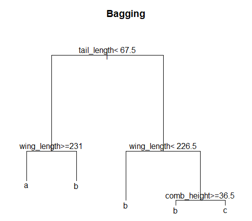

처음에는 tail_length를 기준으로 분할한 뒤 그 다음에는 wign_length를 기준으로 분할하고, 제일 마지막에는 상대적으로 중요도가 낮았던 comb_height을 기준으로 분할했다.

모델 성능 평가

pred는 예측값(class) 외에도 다양한 결과가 입력된 리스트 형태이다.

> pred <- predict(bag, newdata=test, type='class')

> str(pred)
List of 6
 $ formula  :Class 'formula'  language breeds ~ .
  .. ..- attr(*, ".Environment")=<environment: R_GlobalEnv> 
 $ votes    : num [1:60, 1:3] 100 100 100 100 100 23 100 100 99 100 ...
 $ prob     : num [1:60, 1:3] 1 1 1 1 1 0.23 1 1 0.99 1 ...
 $ class    : chr [1:60] "a" "a" "a" "a" ...
 $ confusion: 'table' int [1:3, 1:3] 19 1 0 2 16 2 0 2 18
  ..- attr(*, "dimnames")=List of 2
  .. ..$ Predicted Class: chr [1:3] "a" "b" "c"
  .. ..$ Observed Class : chr [1:3] "a" "b" "c"
 $ error    : num 0.117

> test$pred <- as.factor(pred$class)

> library(caret)
> confusionMatrix(test$pred, test$breeds)
Confusion Matrix and Statistics

          Reference
Prediction  a  b  c
         a 19  2  0
         b  1 16  2
         c  0  2 18

Overall Statistics
                                          
               Accuracy : 0.8833          
                 95% CI : (0.7743, 0.9518)
    No Information Rate : 0.3333          
    P-Value [Acc > NIR] : < 2.2e-16       
                                          
                  Kappa : 0.825           
                                          
 Mcnemar's Test P-Value : NA              

Statistics by Class:

                     Class: a Class: b Class: c
Sensitivity            0.9500   0.8000   0.9000
Specificity            0.9500   0.9250   0.9500
Pos Pred Value         0.9048   0.8421   0.9000
Neg Pred Value         0.9744   0.9024   0.9500
Prevalence             0.3333   0.3333   0.3333
Detection Rate         0.3167   0.2667   0.3000
Detection Prevalence   0.3500   0.3167   0.3333
Balanced Accuracy      0.9500   0.8625   0.925

> pred$confusion
               Observed Class
Predicted Class  a  b  c
              a 19  2  0
              b  1 16  2
              c  0  2 18