Pytorch_07_rnn

이번시간에는 Pytorch에서 RNN을 적용하는 방법에 대해서 알아보겠습니다.

코드예제

import numpy as np
from sklearn.metrics import accuracy_score
import torch
import torch.nn as nn
import torch.optim as optim
import random 

random.seed(333)
np.random.seed(333)
torch.manual_seed(333) #토치 고정
torch.cuda.manual_seed(333) #gpu 고정

# USE_CUDA = torch.cuda.is_available()
# DEVICE = torch.device('cuda:0'if USE_CUDA else 'cpu')
# print('torch' , torch.__version__, '사용DEVICE : ', DEVICE)

DEVICE = 'cuda:0' if torch.cuda.is_available else 'cpu'
print(DEVICE)


#1. 데이터 
datasets = np.array([1,2,3,4,5,6,7,8,9,10])

x = np.array([[1,2,3],
             [2,3,4],
             [3,4,5],
             [4,5,6],
             [5,6,7],
             [6,7,8],
             [7,8,9]])

y = np.array([4,5,6,7,8,9,10])

print(x.shape, y.shape) #(7, 3) (7,)

x = x.reshape(x.shape[0], x.shape[1], 1)
print(x.shape) #(7, 3, 1)

x = torch.FloatTensor(x).to(DEVICE)
y = torch.FloatTensor(y).to(DEVICE)
print(x.shape, y.size()) #torch.Size([7, 3, 1]) torch.Size([7])

from torch.utils.data import TensorDataset #x, y 합친다
from torch.utils.data import DataLoader # batch정의

train_set = TensorDataset(x,y)

train_loader = DataLoader(train_set, batch_size=2, shuffle=True)

# aaa = iter(train_loader)
# bbb = next(aaa) #aaa.next()

# print(bbb) 
# # [tensor([[[5.],
# #          [6.],
# #          [7.]],

# #         [[6.],
# #          [7.],
# #          [8.]]], device='cuda:0'), tensor([8., 9.], device='cuda:0')]
# print(bbb[0].size()) #torch.Size([2, 3, 1])

#2. 모델
class RNN(nn.Module):
    def __init__(self):
        super().__init__()
        self.cell = nn.RNN(input_size=1, #피쳐갯수
                           hidden_size=32, #아웃풋 노드의 갯수
                        #    num_layers=1,
                           batch_first=True, # batch first를 적용하지 않으면 연산의 결과가 (2, 3, 1) -> (3 ,2, 1)로 출력됨
                           ) # (3, N, 1) -> (N, 3, 1) -> (N, 3, 32)
        self.fc1 = nn.Linear(3*32, 16) # (N, 3*32) -> (N,16)
        self.fc2 = nn.Linear(16, 8) # (N, 16) -> (N, 8)
        self.fc3 = nn.Linear(8, 1) # (N, 8) -> (N, 1)
        self.relu = nn.ReLU()
        self.dropout = nn.Dropout()
        
    def forward(self, x):
        #model.add(SimpleRNN(32, input_shape=(3,1)))
        # x, hidden_state = self.cell(x)
        x, h0 = self.cell(x)
        # x, _ = self.cell(x)
        x = self.relu(x)
        
        x = x.reshape(-1, 3*32)
        x = self.fc1(x)
        x = self.relu(x)
        x = self.fc2(x)
        x = self.fc3(x)
        return x

model = RNN().to(DEVICE)

from torchsummary import summary
summary(model, (3, 1))   

코드설명

데이터 전처리

데이터 파트는 크게 변동되는 부분이 없어 위의 코드를 참고시길 바랍니다.

모델 구성

class RNN(nn.Module):
    def __init__(self):
        super().__init__()
        self.cell = nn.RNN(input_size=1, #피쳐갯수
                           hidden_size=32, #아웃풋 노드의 갯수
                        #    num_layers=1,
                           batch_first=True, # batch first를 적용하지 않으면 연산의 결과가 (2, 3, 1) -> (3 ,2, 1)로 출력됨
                           ) # (3, N, 1) -> (N, 3, 1) -> (N, 3, 32)
        self.fc1 = nn.Linear(3*32, 16) # (N, 3*32) -> (N,16)
        self.fc2 = nn.Linear(16, 8) # (N, 16) -> (N, 8)
        self.fc3 = nn.Linear(8, 1) # (N, 8) -> (N, 1)
        self.relu = nn.ReLU()
        self.dropout = nn.Dropout()

• RNN이라는 Class를 선언합니다.

• RNN은 기존과 마찬가지로 Module을 불러옵니다.

• self.cell 은 nn.RNN에 input되는 값들은 다음과 같습니다.
  input_size = 1 (피쳐의 갯수)
  hidden_size = 32 (아웃풋 노드의 갯수)
  batch_first = True (batch_first를 적용하지 않으면 (2, 3, 1) -> (3 ,2, 1)로 출력됨)

• self.fc1의 nn.Linear (3*32, 16)로 설정하는 이유는 keras의 RNN과 다르게 output이 자동적으로 2차원의 shape으로 변환되지 않습니다. 따라서 reshape를 해줘야합니다.

• 이외의 것들은 기존의 내용과 동일합니다.

  def forward(self, x):
        #model.add(SimpleRNN(32, input_shape=(3,1)))
        # x, hidden_state = self.cell(x)
        x, h0 = self.cell(x)
        x = self.relu(x)
        x = x.reshape(-1, 3*32)
        x = self.fc1(x)
        x = self.relu(x)
        x = self.fc2(x)
        x = self.fc3(x)
        return x

• Pytorch의 RNN에서는 기존의 RNN과 다르게 hidden_state가 명시됩니다.

• 처음 input되는 hidden state의 값은 0입니다. 그 값이 input될 x값과 연산됩니다. 이 부분은 RNN 개념설명 부분에서 면밀하게 살펴보겠습니다.

• reshape를 위해서 x.reshape( -1, 3*32)를 선언합니다.

model = RNN().to(DEVICE)
from torchsummary import summary
summary(model, (3, 1))   

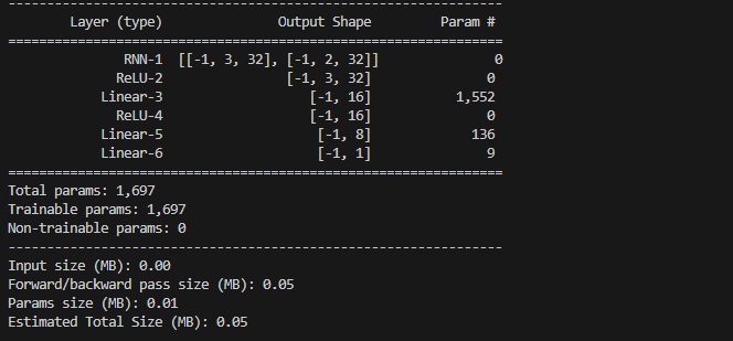
• 모델을 선언해준 뒤 summary했을 때에 아래와 같습니다.

• shape이 두가지로 보이는 것을 확인할 수 있습니다.

• 이것은 hidden shape입니다.