이번 시간에는 Pytorch에서 LSTM을 적용하는 방법에 대하여 알아보겠습니다.
코드예제
import numpy as np
from sklearn.metrics import accuracy_score
import torch
import torch.nn as nn
import torch.optim as optim
import random

random.seed(333)
np.random.seed(333)
torch.manual_seed(333) #토치 고정
torch.cuda.manual_seed(333) #gpu 고정

# USE_CUDA = torch.cuda.is_available()
# DEVICE = torch.device('cuda:0'if USE_CUDA else 'cpu')
# print('torch' , torch.__version__, '사용DEVICE : ', DEVICE)

DEVICE = 'cuda:0' if torch.cuda.is_available else 'cpu'
print(DEVICE)


#1. 데이터
datasets = np.array([1,2,3,4,5,6,7,8,9,10])

x = np.array([[1,2,3],
             [2,3,4],
             [3,4,5],
             [4,5,6],
             [5,6,7],
             [6,7,8],
             [7,8,9]])

y = np.array([4,5,6,7,8,9,10])

print(x.shape, y.shape) #(7, 3) (7,)

x = x.reshape(x.shape[0], x.shape[1], 1)
print(x.shape) #(7, 3, 1)

x = torch.FloatTensor(x).to(DEVICE)
y = torch.FloatTensor(y).to(DEVICE)
print(x.shape, y.size()) #torch.Size([7, 3, 1]) torch.Size([7])

from torch.utils.data import TensorDataset #x, y 합친다
from torch.utils.data import DataLoader # batch정의

train_set = TensorDataset(x,y)

train_loader = DataLoader(train_set, batch_size=2, shuffle=True)

# aaa = iter(train_loader)
# bbb = next(aaa) #aaa.next()

# print(bbb)
# # [tensor([[[5.],
# #          [6.],
# #          [7.]],

# #         [[6.],
# #          [7.],
# #          [8.]]], device='cuda:0'), tensor([8., 9.], device='cuda:0')]
# print(bbb[0].size()) #torch.Size([2, 3, 1])

#2. 모델
class LSTM(nn.Module):
    def __init__(self):
        super().__init__()
        self.cell = nn.LSTM(input_size=1, #피쳐갯수
                           hidden_size=32, #아웃풋 노드의 갯수
                           num_layers=1, # 전설 : 디폴트 아니면 3, 5 좋아.
                           batch_first=True, # batch first를 적용하지 않으면 연산의 결과가 (2, 3, 1) -> (3 ,2, 1)로 출력됨

                           ) # (3, N, 1) -> (N, 3, 1) -> (N, 3, 32)
        self.fc1 = nn.Linear(3*32, 16) # (N, 3*32) -> (N,16)
        self.fc2 = nn.Linear(16, 8) # (N, 16) -> (N, 8)
        self.fc3 = nn.Linear(8, 1) # (N, 8) -> (N, 1)
        self.relu = nn.ReLU()
        self.dropout = nn.Dropout()

    def forward(self, x, h0, c0):
        #model.add(LSTM(32, input_shape=(3,1)))
        # if h0 is None:
        h0 = torch.zeros(1, x.size(0), 32).to(DEVICE) #(num_layers, bath_size, hidden_size)
        c0 = torch.zeros(1, x.size(0), 32).to(DEVICE) #(num_layers, bath_size, hidden_size)

        # x, hidden_state = self.cell(x)
        x, (hn, cn) = self.cell(x, (h0, c0))
        # x, _ = self.cell(x)
        x = self.relu(x)
        x = x.contiguous()
        x = x.view(-1, 3*32)
        x = self.fc1(x)
        x = self.relu(x)
        x = self.fc2(x)
        x = self.fc3(x)
        return x

model = LSTM().to(DEVICE)

# from torchsummary import summary
# summary(model, (3, 1))


#3. 컴파일 훈련

criterion = nn.MSELoss()
optimizer = optim.Adam(model.parameters(), lr=0.01)

def train(model, criterion, optimizer, loader):
    epoch_loss = 0

    model.train()

    for x_batch, y_batch in loader:
        x_batch, y_batch = x_batch.to(DEVICE), y_batch.to(DEVICE).float().view(-1, 1) #백터형태를 매트릭스로 변환

        optimizer.zero_grad() # 기울기 0으로 초기화
        h0 = torch.zeros(1, x_batch.size(0), 32).to(DEVICE)
        c0 = torch.zeros(1, x_batch.size(0), 32).to(DEVICE)

        hypothesis = model(x_batch, h0, c0) #hidden과 cell state 튜플로 묶을 필요 없음 여기선
        loss = criterion(hypothesis, y_batch) # 여기까지 순전파

        loss.backward() # 기울기 계산 역전파 시작
        optimizer.step() # 가중치 갱신

        epoch_loss += loss.item()
    return epoch_loss / len(loader)


def evaluate(model, criterion, loader):
    epoch_loss = 0

    model.eval()

    with torch.no_grad():

        for x_batch, y_batch in loader:
            x_batch, y_batch = x_batch.to(DEVICE), y_batch.to(DEVICE).float().view(-1, 1) #백터형태를 매트릭스로 변환

            # optimizer.zero_grad() # 기울기 0으로 초기화
            h0 = torch.zeros(1, x_batch.size(0), 32).to(DEVICE)
            c0 = torch.zeros(1, x_batch.size(0), 32).to(DEVICE)

            hypothesis = model(x_batch, h0, c0)
            loss = criterion(hypothesis, y_batch) # 여기까지 순전파

            # loss.backward() # 기울기 계산 역전파 시작
            # optimizer.step() # 가중치 갱신

            epoch_loss += loss.item()
    return epoch_loss / len(loader)

for epoch in range(1, 1001):
    loss = train(model, criterion, optimizer, train_loader)

    if epoch %20 == 0 : # 20에포마다 학습
        print('epoch: {}, loss: {}'.format(epoch, loss))

#4. 평가 예측

x_predict = np.array([[8,9,10]])

def predict(model, data):
    model.eval()
    with torch.no_grad():
        data = torch.FloatTensor(data).unsqueeze(2).to(DEVICE) # (1,3) -> (1,3,1)
        h0 = torch.zeros(1, data.size(0), 32).to(DEVICE)
        c0 = torch.zeros(1, data.size(0), 32).to(DEVICE)

        y_predict = model(data, h0, c0)
    return y_predict.cpu().numpy()

y_predict = predict(model, x_predict)
print('---------------------------------------------------------')
print(y_predict)
print('---------------------------------------------------------')
print(y_predict[0])
print('---------------------------------------------------------')
print(f'{x_predict[0]}의 예측값 : {y_predict[0][0]}')
코드 설명
모델 구성
#2. 모델
class LSTM(nn.Module):
    def __init__(self):
        super().__init__()
        self.cell = nn.LSTM(input_size=1, #피쳐갯수
                           hidden_size=32, #아웃풋 노드의 갯수
                           num_layers=1, # 전설 : 디폴트 아니면 3, 5 좋아.
                           batch_first=True, # batch first를 적용하지 않으면 연산의 결과가 (2, 3, 1) -> (3 ,2, 1)로 출력됨
                           ) # (3, N, 1) -> (N, 3, 1) -> (N, 3, 32)
        self.fc1 = nn.Linear(3*32, 16) # (N, 3*32) -> (N,16)
        self.fc2 = nn.Linear(16, 8) # (N, 16) -> (N, 8)
        self.fc3 = nn.Linear(8, 1) # (N, 8) -> (N, 1)
        self.relu = nn.ReLU()
        self.dropout = nn.Dropout()
LSTM을 사용해주기 위해서 기본적으로 모델 구성하는 코드는 RNN과 크게 변형된 것은 없습니다. 먼저 RNN → LSTM으로 교체해주겠습니다.
def forward(self, x, h0, c0):
        #model.add(LSTM(32, input_shape=(3,1)))
        # if h0 is None:
        h0 = torch.zeros(1, x.size(0), 32).to(DEVICE) #(num_layers, bath_size, hidden_size)
        c0 = torch.zeros(1, x.size(0), 32).to(DEVICE) #(num_layers, bath_size, hidden_size)# x, hidden_state = self.cell(x)
        x, (hn, cn) = self.cell(x, (h0, c0))
        # x, _ = self.cell(x)
        x = self.relu(x)
        x = x.contiguous()
        x = x.view(-1, 3*32)
        x = self.fc1(x)
        x = self.relu(x)
        x = self.fc2(x)
        x = self.fc3(x)
        return x
그런데 forward 함수를 정의하는 부분에서 이전과 다르게 hidden state외에 추가로 c0이 확인됩니다. 이를 이해하기 위해선 LSTM의 구조에 대하여 살펴볼 필요가 있습니다.
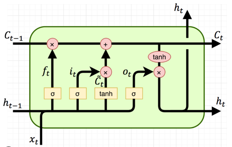
LSTM의 구조를 확인할 때에 Hidden state와 Cell state가 확인됩니다.
input된 Cell state와 Hidden state는 X값과 연산되어 Ct와 Ht를 아웃풋하게 됩니다.
위 내용을 고려하며 forward 함수를 살펴보겠습니다.
-
h0 변수에 torch.zero 함수를 사용하여 가중치를 0으로 초기화해줍니다.
-
(1, x.size(0), 32)는 (num_layers, bath_size, hidden_size)입니다.
-
x데이터는 numpy형태입니다. 따라서 Tensor 형태로 변환해줍니다.
-
x, (hn, cn)는 cell 함수에 x와 튜플 형태의 (h0, c0)을 넣어줍니다.
-
이후 선언한 함수를 거쳐 최종 x를 return해줍니다.
model = LSTM().to(DEVICE)
- 모델은 LSTM을 GPU로 실행합니다.
컴파일 훈련
def train(model, criterion, optimizer, loader):
    epoch_loss = 0
    model.train()
    for x_batch, y_batch in loader:
        x_batch, y_batch = x_batch.to(DEVICE), y_batch.to(DEVICE).float().view(-1, 1) #백터형태를 매트릭스로 변환
        optimizer.zero_grad() # 기울기 0으로 초기화
        h0 = torch.zeros(1, x_batch.size(0), 32).to(DEVICE)
        c0 = torch.zeros(1, x_batch.size(0), 32).to(DEVICE)
        hypothesis = model(x_batch, h0, c0) #hidden과 cell state 튜플로 묶을 필요 없음 여기선
        loss = criterion(hypothesis, y_batch) # 여기까지 순전파
        loss.backward() # 기울기 계산 역전파 시작
        optimizer.step() # 가중치 갱신
        epoch_loss += loss.item()
    return epoch_loss / len(loader)
- 컴파일 단계에서 마찬가지로 h0과 c0 변수를 추가합니다.
- hypothesis는 model에 x_batch와 h0, c0을 넣어 예측한 y 값입니다.
- train 단계에선 h0과 c0을 튜플로 묶지 않아도 됩니다.
- loss.backward를 통해 역전파를 진행합니다.
- optimzer.step을 통해 가중치를 갱신합니다.
- eopch_loss에 loss가 누적됩니다.
- 누적 된 loss를 loader의 길이만큼 나눠 return해줍니다.
def evaluate(model, criterion, loader):
    epoch_loss = 0
    model.eval()
    with torch.no_grad():
        for x_batch, y_batch in loader:
            x_batch, y_batch = x_batch.to(DEVICE), y_batch.to(DEVICE).float().view(-1, 1) #백터형태를 매트릭스로 변환
            # optimizer.zero_grad() # 기울기 0으로 초기화
            h0 = torch.zeros(1, x_batch.size(0), 32).to(DEVICE)
            c0 = torch.zeros(1, x_batch.size(0), 32).to(DEVICE)
            hypothesis = model(x_batch, h0, c0)
            loss = criterion(hypothesis, y_batch) # 여기까지 순전파
            # loss.backward() # 기울기 계산 역전파 시작
            # optimizer.step() # 가중치 갱신
            epoch_loss += loss.item()
    return epoch_loss / len(loader)
-
with torch.no_grad(): 를 통해 이후의 과정에선 기울기가 갱신되지 않습니다.
-
x_batch와 y_batch는 numpy형태이므로 Tensor형태로 변환해줍니다.
-
hidden state와 cell state 정의해줍니다.
-
hypothesis는 model에 x_batch와 정의된 hidden state와 cell state를 입력하여 계산한 값입니다.
for epoch in range(1, 1001):
    loss = train(model, criterion, optimizer, train_loader)
    if epoch %20 == 0 : # 20에포마다 학습
        print('epoch: {}, loss: {}'.format(epoch, loss))
-
for문의 반복 횟수는 1000번 입니다.
-
앞서 선언한 train 함수에 model, criterion, optimizer, train loader를 적용하여 훈련을 진행합니다.
-
epoch를 20으로 나눌때 나머지가 0일때 즉 20에포마다 epoch와 loss 값을 출력합니다.
평가예측
#4. 평가 예측
x_predict = np.array([[8,9,10]])
def predict(model, data):
    model.eval()
    with torch.no_grad():
        data = torch.FloatTensor(data).unsqueeze(2).to(DEVICE) # (1,3) -> (1,3,1)
        h0 = torch.zeros(1, data.size(0), 32).to(DEVICE)
        c0 = torch.zeros(1, data.size(0), 32).to(DEVICE)
        y_predict = model(data, h0, c0)
    return y_predict.cpu().numpy()
y_predict = predict(model, x_predict)
-
x_predict는 예측 과정에서 input될 x데이터 값입니다.
-
x 데이터의 shape는 (1,3)이므로 model에서 요구하는 3차원의 shape로 변환합니다.
-
또한 torch 모델에 맞게 Tensor형태로 변환합니다.
-
y_predict는 model에 변환한 data와 hidden state, cell state 통해 예측한 값입니다.
-
y_predict를 numpy형태로 최종 return 해줍니다.
y_predict = predict(model, x_predict)
print('---------------------------------------------------------')
print(y_predict)
print('---------------------------------------------------------')
print(y_predict[0])
print('---------------------------------------------------------')
print(f'{x_predict[0]}의 예측값 : {y_predict[0][0]}')
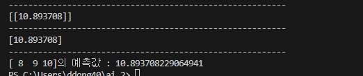
최종 예측값은 위와 같이 도출 됩니다.