Theory
검정력 (Power) 이란 특정 표본 조건 (size and variability) 에서 특정한 효과 크기 (effect size) 를 알아낼 수 있는 확률을 의미한다. 실제 차이가 크면 클수록 그것을 밝혀낼 가능성도 따라서 커질 것이고, 그 차이가 작을수록 더 많은 데이터가 필요하게 된다.
Example)
25타석에서 3할 3푼 타자와 2할 타자를 구분할 수 있을 확률은 0.75이다.
→ n=25일 때의 실험은 0.130의 효과 크기에 대해 0.75(75%)의 검정력을 가진다고 볼 수 있다.
검정력의 사전적 정의
- 대립가설이 사실일 때, 이를 사실로서 결정할 확률
- 검정력이 90%라고 하면, 대립가설이 사실임에도 불구하고 귀무가설을 채택할 확률(2종 오류, β error) 의 확률은 10%이다.
- 검정력 = 1 - β
검졍력을 왜 알아야 하는가?
- 검정력 계산의 주된 용도는 표본크기가 어느 정도 필요한가를 추정하는 것임.
- '효과크기'가 표본크기를 좌우함! (기대하는 효과 크기가 작을수록 표본사이즈가 증가되어야 함)
검정력/표본크기 계산의 4요소
- 표본크기 (Sample size)
- 탐지하고자 하는 효과크기 (Effect size)
- 가설검정을 위한 유의수준 (Significance level)
- 검정력 (Power)
Ref) 검정력 계산에 관한 수식
Practice (MATLAB)
Ref) MATLAB sampsizepwr
sampsizepwr
sampsizepwr computes the sample size, power, or alternative parameter value for a hypothesis test, given the other two value. For example, you can compute the sample size required to obtain a particular power for a hypothesis test, given the parameter value of the alternative hypothesis.
Example 1
A company runs manufacturing process that fills empty bottles with 100 mL of liquid. To monitor quality, the company randomly selects several bottles and measures the volume of liquid inside.
Determine the sample size the compnay must use for a t-test to detect a difference between 100 mL and 102 mL with a power of 0.80.
nout = sampsizepwr('t', [100 5], 102, 0.80)
The compnay must test 52 bottles to detect the difference between a mean volume of 100 mL and 102 mL with a power of 0.80.
Generate a power curve to visualize how the sample size affects the power of test.
nn = 1:100;
pwrout =  sampsizepwr('t', [100 5], 102, [], nn);

figure;
plot(nn, pwrout, 'b-', nout, 0.8, 'ro')
title('Power versus Sample Size')
xlabel('Sample Size')
ylabel('Power')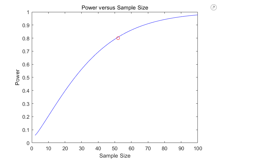
Example 2
An employee wants to buy a house near her office. She decides to eliminate from consideration any house that has a mean morning commute time greater than 20 minutes. The null hypothesis for this right-sided test is H0: μ = 20, and the alternative hypothesis is HA: μ > 20. The selected significance level is 0.05.
To determine the mean commute time, the employee takes a test drive from the house to her office during rush hour every morning for one week, so her total sample size is 5. She assumes that the standard deviation, σ, is equal to 5.
The employee decides that a true mean commute time of 25 minutes is too different from her targeted 20-minute limit, so she wants to detect a significant departure if the true mean is 25 minutes. Find the probability of incorrectly concluding that the mean commute time is no greater than 20 minutes.
Compute the power of the test, and then subtract the power from 1 to obtain β.
power = sampsizepwr('t',[20 5],25,[],5,'Alpha',0.05,'Tail','right')
beta = 1 - power
The employee decides that this risk is too high, and she wants no more than a 0.01 probability of reaching an incorrect conclusion. Calculate the number of test drives the employee must take to obtain a power of 0.99.
nout = sampsizepwr('t',[20 5],25,0.99,[],'Tail','right')The results indicate that she must take 18 test drives from a candidate house to achieve this power level.
The employee decides that she only has time to take 10 test drives. She also accepts a 0.05 probability of making an incorrect conclusion. Calculate the smallest true parameter value that produces a detectable difference in mean commute time.
p1out = sampsizepwr('t',[20 5],[],0.95,10,'Tail','right')
Given the employee's target power level and sample size, her test detects a significant difference from a mean commute time of at least 25.6532 minutes.