1.학습한 내용

Numpy

Numpy의 소개
-NumPy(Numerical Python)는 파이썬에서 과학적 계산을 위한 핵심 라이브러리이다. NumPy는 다차원 배열 객체와 배열과 함께 작동하는 도구들을 제공한다. 하지만 NumPy 자체로는 고수준의 데이터 분석 기능을 제공하지 않기 때문에 NumPy 배열과 배열 기반 컴퓨팅의 이해를 통해 pandas와 같은 도구를 좀 더 효율적으로 사용하는 것이 필요하다.

ndarray 생성

-array 함수를 사용하여 배열 생성하기

import numpy as np
arr = np.array([1,2,3,4])

-int a는 정수를 할당하는 것
-a는 빈칸으로 되어있으나 메모리 찌꺼기 값은 남아있기때문에 다르게 동작될 수 있다.
때문에 항상 int a=0으로 만들어 준다. 그 명령어가 파이썬에서 zeros
-0은 계산이 가능하지만 Null은 진공과 같은 상태로 계산되지 않는 차이가 있다.

np.zeros((3,3))

-때에 따라 1로 배열되는 함수가 필요할땐 ones 사용

• 1. = 뒤에 0이 있다는 의미

np.ones((3,3))

• 속에 아무거나 채워달라는 명령 empty
• 나오는 값들이 일종의 찌꺼기(garbage = 다른 데이터들이 흘리고간 데이터)
• 코딩을 하기위해서 컴퓨터의 하드웨어적인 구조들을 잘 알 필요가 있다.

np.empty((4,4))

• arange = 범위, 보통 [0,1,2,3,4] 사용했었지만 arange를 사용하면 간단히 할 수 있다.

np.arange(10)

ndarray 배열의 모양, 차수, 데이터타입 확인하기

arr = np.array([[1,2,3],[4,5,6]])

• shape 모양 확인
  arr.shape

• 몇 차원 데이터인가 ndim
  arr.ndim

• 데이터타입
  arr.dtype

• float = 실수형
  arr_float = arr.astype(np.float64)

• numpy는 내부적으로 연산이 빠르고 다양하게 가능하다

• arr 통째로 사칙연산 가능, 연산자를 사용해도 되고 직접 연산해도 된다.

• Numpy 배열의 연산은 연산자 (+,-,*,/)나 함수(add, subtract, multiply, divide)로 가능하다.
  arr1 = np.array([[1,2],[3,4]])
  arr2 = np.array([[5,6],[7,8]])

• 예시
  arr3 = arr1 + arr2
  print(arr3)
  arr3 = np.add(arr1,arr2)
  print(arr3)

arr3 = arr1 * arr2
print(arr3)
arr3 = np.multiply(arr1,arr2)
print(arr3)

ndarray 배열 슬라이싱 하기

-ndarray 배열 슬라이싱 하기

• 배열 슬라이싱
  arr = np.array([[1,2,3],[4,5,6],[7,8,9]])

• :2 => 앞에 뭔가 생략되어 있음 = 처음부터 2개를 가지고 오겠다는 의미

• 1:3 => 1부터 3전에 까지의 조건을 만족하는 값을 의미
  arr_1 = arr[:2,1:3]
  print(arr_1)

• :5 => 처음부터 5까지를 가지고 오겠다는 의미

• 5: => 5부터 끝까지를 가지고 오겠다는 의미

• 0:8 => 0~8까지

• 0:8:3 => 세번째 값은 증가 값을 의미
  arr_int = np.arange(10)
  print(arr_int[:5])
  print(arr_int[5:])
  print(arr_int[0:8:3])
  print(arr_int[:])

• 열0 1 2 행0 1 2 = 열의 세로 0번째, 행의 가로 2번째 값
  print(arr[0,2])
  print(arr[2,0])

arr = np.array([[1,2,3,],[4,5,6]])

• idx 라는 새로운 변수
  idx = arr > 3
  print(idx)
• arr[idx]는 참인 값만 출력된다
  print(arr[idx])

Wine Quality 데이터

• 레드와인 화이트와인 두 개의 데이터 셋
• 각각의 데이터 셋 안에는 12가지의 서로 다른 조건들이 있다.

redwine = np.loadtxt(fname = 'samples/winequality-red.csv',
delimiter = ';', (구별자)
skiprows = 1) (첫줄은 무시하겠다)

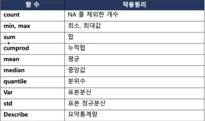
print(redwine.sum()) # 합
print(redwine.mean()) # 평균

print(redwine.mean(axis=0)) #axis = 각각의 축(열)

• 내가 원하는 항목의 값만 구할 수 있다
  print(redwine[:,0].mean())

redwine.max(axis=0): redwine 데이터 셋의 열별(변수별) 최대값
redwine.min(axis=0): redwine 데이터 셋의 열별(변수별) 최소값

Pandas

-Pandas는 쉽고 직관적인 관계형 또는 분류된 데이터로 작업할 수 있도록 설계된 빠르고 유연하며 표현이 풍부한 데이터 구조를 제공하는 Python 패키지

엑셀 칼럼(기둥) = Series(1차원)
엑셀 표 = DataFrame(2차원)

자료구조 : Series 와 DataFrame

Dataframe
Pandas에서 제공하는 데이터 자료구조는 Series와 Dataframe 두가지가 존재하는데 Series는 시계열과 유사한 데이터로서 index와 value가 존재하고 Dataframe은 딕셔너리데이터를 매트릭스 형태로 만들어 준 것 같은 frame을 가지고 있다. 이런 데이터 구조를 통해 시계열, 비시계열 데이터를 통합하여 다룰 수 있다.

Series

import pandas as pd
from pandas import Series, DataFrame
fruit = Series([2500,3800,1200,6000],
index=['apple','banana','pear','cherry'])
(Key + value = dictionaly 타입)
apple 2500
banana 3800
pear 1200
cherry 6000
dtype: int64

print(fruit.values)
print(fruit.index)
[2500 3800 1200 6000]
Index(['apple', 'banana', 'pear', 'cherry'], dtype='object')

fruitData = {'apple':2500,'banana':3800,'pear':1200,'cherry':6000}
fruit = Series(fruitData)

print(type(fruitData))
print(type(fruit))
<class 'dict'>
<class 'pandas.core.series.Series'>

fruit.name = 'fruitPrice'
fruit.index.name = 'fruitName'
fruitName
apple 2500
banana 3800
pear 1200
cherry 6000
Name: fruitPrice, dtype: int64

DataFrame

fruitData = {'fruitName':['apple','banana','cherry','pear'],'fruitPrice':[2500,3800,6000,1200],'num':[10,5,3,8]}
fruitFrame = DataFrame(fruitData)
fruitName fruitPrice num
0 apple 2500 10
1 banana 3800 5
2 cherry 6000 3
3 pear 1200 8

fruitFrame = DataFrame(fruitData, columns = ['fruitPrice','num','fruitName'])\
-칼럼 순서를 지정할 수 있다
fruitPrice num fruitName
0 2500 10 apple
1 3800 5 banana
2 6000 3 cherry
3 1200 8 pear

-한 항목만 뽑아서 보기
fruitFrame['fruitName']
0 apple
1 banana
2 cherry
3 pear
Name: fruitName, dtype: object

-새로운 칼럼을 추가할 때
fruitFrame['Year'] = '2022'
fruitPrice num fruitName Year
0 2500 10 apple 2022
1 3800 5 banana 2022
2 6000 3 cherry 2022
3 1200 8 pear 2022

-각각의 값을 추가, 수정하고 싶을 때
-index를 지정해주지 않으면 자동으로 0부터 지정된다.
variable = Series([4,2,1],index=[0,2,3])
0 4
2 2
3 1
dtype: int64

fruitFrame['stock'] = variable
fruitPrice num fruitName Year stock
0 2500 10 apple 2022 4.0
1 3800 5 banana 2022 NaN
2 6000 3 cherry 2022 2.0
3 1200 8 pear 2022 1.0

fruit = Series([2500,3800,1200,6000],index=['apple','banana','pear','cherry'])
apple 2500
banana 3800
pear 1200
cherry 6000
dtype: int64

-banana를 지우기, 삭제명령 = drop, 원본을 지우진 못함, 삭제된 사본을 돌려주는것.
new_fruit = fruit.drop('banana')
apple 2500
pear 1200
cherry 6000
dtype: int64

-index를 name 지정하기
fruitName = fruitData['fruitName']['apple', 'banana', 'cherry', 'pear']

fruitFrame = DataFrame(fruitData,
index=fruitName,
columns=['fruitPrice','num'])
fruitPrice num
apple 2500 10
banana 3800 5
cherry 6000 3
pear 1200 8

-apple,cherry 삭제
fruitFrame2 = fruitFrame.drop(['apple','cherry'])
fruitPrice num
banana 3800 5
pear 1200 8

-num칼럼을 삭제
fruitFrame3 = fruitFrame.drop('num',axis=1)
fruitPrice
apple 2500
banana 3800
cherry 6000
pear 1200

-항목 추출하기, ':'는 a:b a에서 b까지를 의미, [0.1]로도 되지만 부정확하기 때문에 지정한txt사용
fruit['apple':'pear']
apple 2500
banana 3800
pear 1200
dtype: int64

fruitFrame['apple':'banana']
fruitPrice num
apple 2500 10
banana 3800 5

fruit1 = Series([5,9,10,3],index=['apple','banana','cherry','pear'])
fruit2 = Series([3,2,9,5,10],index=['apple','orange','banana','cherry','mango'])
-다른 두개의 값을 처리
-같은 index는 연산이 되지만 한 쪽에만 있는 것들은 NAN이 뜬다.
-양쪽이 똑같이 존재해야 그 값이 나온다.
fruit1 + fruit2
apple 8.0
banana 18.0
cherry 15.0
mango NaN
orange NaN
pear NaN
dtype: float64

fruitData1 = {'Ohio' : [4,8,3,5],'Texas' : [0,1,2,3]}
fruitFrame1 = DataFrame(fruitData1,columns=['Ohio','Texas'],index = ['apple','banana','cherry','pear'])
fruitData2 = {'Ohio' : [3,0,2,1,7],'Colorado':[5,4,3,6,0]}
fruitFrame2 = DataFrame(fruitData2,columns =['Ohio','Colorado'],index = ['apple','orange','banana','cherry','mango']

fruitFrame1
Ohio Texas
apple 4 0
banana 8 1
cherry 3 2
pear 5 3

fruitFrame2
Ohio Colorado
apple 3 5
orange 0 4
banana 2 3
cherry 1 6
mango 7 0

fruitFrame1 + fruitFrame2
Colorado Ohio Texas
apple NaN 7.0 NaN
banana NaN 10.0 NaN
cherry NaN 4.0 NaN
mango NaN NaN NaN
orange NaN NaN NaN
pear NaN NaN NaN

• 데이터 정렬(순서대로)
  fruit.sort_values()
  pear 1200
  apple 2500
  banana 3800
  cherry 6000
  dtype: int64

-비싼값 순서대로 정렬
fruit.sort_values(ascending=False)
cherry 6000
banana 3800
apple 2500
pear 1200
dtype: int64

-index를 알파벳 순서대로
fruit.sort_index()
apple 2500
banana 3800
cherry 6000
pear 1200
dtype: int64

fruitFrame.sort_values(by=['fruitPrice','num'])
fruitPrice num
pear 1200 8
apple 2500 10
banana 3800 5
cherry 6000 3

상관계수, 그룹

german = pd.read_csv('german_credit.csv')
list(german.columns.values)
'Creditability',
'Account Balance',
'Duration of Credit (month)',
'Payment Status of Previous Credit',
'Purpose',
'Credit Amount',
'Value Savings/Stocks',
'Length of current employment',
'Instalment per cent',
'Sex & Marital Status',
'Guarantors',
'Duration in Current address',
'Most valuable available asset',
'Age (years)',
'Concurrent Credits',
'Type of apartment',
'No of Credits at this Bank',
'Occupation',
'No of dependents',
'Telephone',
'Foreign Worker'

erman_sample = german[['Creditability','Duration of Credit (month)','Purpose','Credit Amount']]
german_sample.describe() (전체 요약정보)
Creditability Duration of Credit (month) Purpose Credit Amount
count 1000.000000 1000.000000 1000.000000 1000.00000
mean 0.700000 20.903000 2.828000 3271.24800
std 0.458487 12.058814 2.744439 2822.75176
min 0.000000 4.000000 0.000000 250.00000
25% 0.000000 12.000000 1.000000 1365.50000
50% 1.000000 18.000000 2.000000 2319.50000
75% 1.000000 24.000000 3.000000 3972.25000
max 1.000000 72.000000 10.000000 18424.00000

-상관 계수 뽑기
-(+)양의 상관관계 = 부채의 증가 = 리치 값 증가
-(-)음의 상관관계 = 부동산 값의 증가 = 리치 값 감소
-상관계수(Correlation)
german_sample = german[['Duration of Credit (month)','Credit Amount','Age (years)']]
german_sample.corr() 상관계수
Duration of Credit (month) Credit Amount Age (years)
Duration of Credit (month) 1.000000 0.624988 -0.037550
Credit Amount 0.624988 1.000000 0.032273
Age (years) -0.037550 0.032273 1.000000

german_sample = german[['Credit Amount','Type of apartment']]
german_grouped = german_sample['Credit Amount'].groupby(
german_sample['Type of apartment'])
german_grouped #전체 데이터를 그룹화했을때 그룹에 대한 정보를 명시해줘야 한다.
german_grouped.mean()

german_sample = german[['Credit Amount','Type of apartment','Purpose']]
german_grouped = german_sample['Credit Amount'].groupby(
[german_sample['Purpose'],
german_sample['Type of apartment']])

상관관계와 공분산

german_sample=german[['Duration of Credit (month)','Credit Amount','Age (years)']]
german_sample.head()

-상관계수
german_sample.corr()

-공분산
german_sample.cov()

핵심기능 Group by

-Group by는 데이터를 구분 할 수 있는 컬럼의 값들을 이용하여 데이터를 여러 기준에 의해 구분 한 뒤 계산 및 순회 등 함수의 계산을 할 수 있는 방법이다. 이런 Group by를 통해 계산하고 반복문을 활용하는 방법을 설명한다.

Group by를 이용한 계산 및 요약 통계

-한 개 그룹 요약 통계

german_sample = german[['Credit Amount','Type of apartment']]
german_grouped = german_sample['Credit Amount'].groupby(german_sample['Type of apartment'])
german_grouped.mean()

german_sample = german[['Credit Amount','Type of apartment','Purpose']]
german_grouped2=german_sample['CreditAmount'].groupby([german_sample['Purpose'],german_sample['Type of apartment']])
german_grouped2.mean()
-group을 두 가지 이상으로 지정하고 싶을 때는 리스트를 통해 그룹을 두 개로 지정하면 된다.

Group간에 반복하기

german=pd.read_csv('german_credit.csv')
german_sample=german[['Type of apartment','Sex & Marital Status','CreditAmount']]

-한 개 그룹 반복
for type , group in german_sample.groupby('Type of apartment'):
print(type)
print(group.head(n=3))

-두개 그룹 반복
for (type,sex) , group in german_sample.groupby(['Type of apartment','Sex & Marital Status']):
print((type,sex))
print(group.head(n=3))

데이터 분석 예제 행성데이터

Seaborn 패키지에서 제공 받을 수 있는 행성 데이터 세트를 사용한다. Seaborn 패키디는 천문학자가 다른 별 주변에서 발견한 행성에대 대한 정보를 제공하며 2014년까지 발견된 1000개 이상의 외계 행성에 대한 세부 정보를 담고 있다.

import seaborn as sns
planets = sns.load_dataset('planets')
planets.shape
planets.head

-dropna() 비여있는 값의 삭제
planets.dropna().describe()

import pandas as pd
births = pd.read_csv('https://raw.githubusercontent.com/jakevdp/data-CDCbirths/master/births.csv')
births
births.head

births['decade'] = (births['year']) // 10 * 10
births
births.pivot_table('births', index='decade', columns='gender', aggfunc='sum')
%matplotlib inline
import matplotlib.pyplot as plt
sns.set()
births.pivot_table('births', index='decade', columns='gender', aggfunc='sum').plot()

2.학습내용 중 어려웠던 점.

-오늘 하루 진도 나간 내용이 어마어마해서 따라가기가 쉽지 않은것 같다. 그리고 마지막에 덜한 부분은 확실히 이해가 좀 덜 가는것 같다.

3.해결방법

-데이터가 많아서 양이 많이 보이긴하지만 작성명령어는 그렇게 많지는 않은 것 같다. 하지만 이게 왜 이런지, 응용이 되는지, 그저 다시 해보는 것 말고는 답이 없는 것 같다.

4.학습소감

-점점 양이 많아짐에 따라 따라가는게 정말 쉽지 않은 것 같지만 치이지말고 할수 있는 한 최대한 따라가야겠다.