📊 sklearn 회귀 모델

📌 sklearn 단순회귀모델 학습과정

• 1. 라이브러리 Import

import numpy as np
import pandas as pd
import matplotlib.pyplot as plt

# feature Scaling을 위한 정규화 모듈
from sklearn.preprocessing import MinMaxScaler

# 회귀 모델
from sklearn.linear_model import LinearRegression

# 모델 성능 평가를 위한 지표 모듈
from sklearn.metrics import r2_score, explained_variance_score, mean_squared_error

---

• 2. 데이터 준비

sample_size = 100
np.random.seed(1)

x = np.random.normal(0, 10, sample_size)
y = np.random.normal(0, 10, sample_size) + x * 30
print(x[:5])
print(y[:5])
# [ 16.24345364  -6.11756414  -5.28171752 -10.72968622   8.65407629]
# [ 482.83232345 -171.28184705 -154.41660926 -315.95480141  248.67317034]

---

• 3. 상관관계 분석

print(np.corrcoef(x, y)[0, 1])
# 0.9993935724865677
# -> 양의 방향으로 매우 강한 관계를 갖는다.

---

• 4. x에 대해 feature Scaling 적용

scaler = MinMaxScaler()
x_scaled = scaler.fit_transform(x.reshape(-1, 1))   # scaler도 sklearn 모델이므로 2차원 matrix로 데이터를 주어야 한다.
print(x_scaled[:5])
# [[0.87492405]
#  [0.37658554]
#  [0.39521325]
#  [0.27379961]
#  [0.70578689]]

---

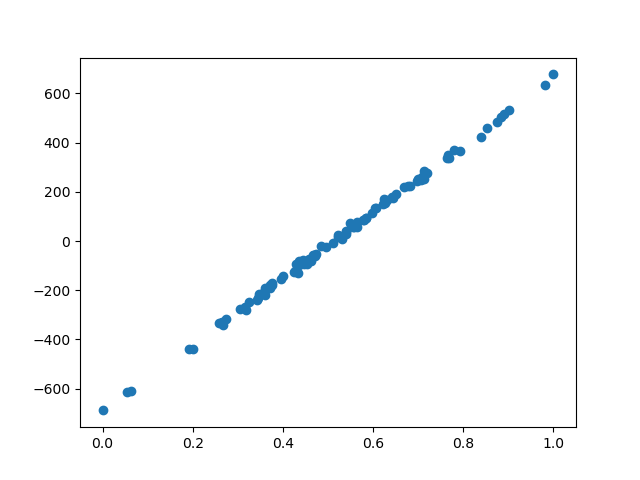
• 5. 상관관계 그래프 그리기

plt.scatter(x_scaled, y)
plt.show()

---

• 6. 모델 생성

model = LinearRegression()
model.fit(x_scaled, y)
y_pred = model.predict(x_scaled)
print('예측값 : ', y_pred[:3])
print('실제값 : ', y[:3])
# 예측값 :  [ 490.32381062 -182.64057041 -157.48540955]
# 실제값 :  [ 482.83232345 -171.28184705 -154.41660926]

---

• 7. 모델 성능 파악용 함수 생성

def RegScore(y, y_pred):
    print('r2_score(결정계수, 설명력) : ', r2_score(y, y_pred))
    print('explained_variance_score(설명분산점수) : ', explained_variance_score(y, y_pred))
    print('mean_squared_error(MSE, 평균제곱오차) : ', mean_squared_error(y, y_pred))

---

• 8. 모델 성능 측정

RegScore(y, y_pred)
# r2_score(결정계수, 설명력) :  0.9987875127274646
# explained_variance_score(설명분산점수) :  0.9987875127274646
# mean_squared_error(MSE, 평균제곱오차) :  86.14795101998743

# [ 모델 성능 결과 분석 ]
# r2_score = 0.998 = 99.8% 설명력이므로 feature가 label을 잘 설명하는 것으로 판단 -> 모델 정확성 만족
# 설명분산점수 = 0.998
# MSE = 86.14

---

• 9. LinearRegression 모델 성능 측정 결과 분석
  - r2score = 0.998 = 99.8% 설명력이므로 feature가 label을 잘 설명하는 것으로 판단
  → 모델 정확성 만족
  - 설명분산점수 = 0.998
  - MSE = 86.14

📌 sklearn 학습, 테스트 데이터 분리

• 사용 목적
  - 데이터가 많을 때, 전체 데이터를 학습 데이터로 사용하게 되면 모델 학습의 과적합이 발생한다. 이로 인해 학습된 모델의 회귀선이 각 데이터에 대해 분산하게 되는데, 이는 데이터의 조그마한 변화에도 예민하게 반응하는 것을 의미한다.

→ 이를 위해 학습 데이터와 검증 데이터를 분리하여 모델 학습에는 학습데이터만 사용하고, 테스트에서는 검증데이터만 사용하여, 모델 과적합을 해소할 수 있다.

• 1. 라이브러리 Import

from sklearn.model_selection import train_test_split

---

• 2. 학습, 테스트 데이터로 분리
  - data : 데이터프레임
  - test_size 속성 : 테스트 데이터 비율
  - random_state 속성 : 시드값 조정

# data : 데이터프레임
# test_size 속성 : 테스트 데이터 비율
# stratify 속성 : 분류 모델에서 범주형 label의 분포를 일정하게 분리하도록 도와줌(label을 속성값으로 준다.)
# random_state : 시드값 조정
train, test = train_test_split(data, test_size=0.3, random_state=41)