-- 01.numpy.ipynb --

NumPy

공식

numpy : 수치적 연산을 위해 최적화된 모듈

파이썬을 활용한 데이터 분석에서 가장 기본!

이 자체로도 많이 쓰이거니와, 앞으로 배울 pandas, 머신러닝 등 수많은 분야에서 기본적으로 사용하는 모듈

파이썬 개발자라면 꼭 익힐 필요 있다

수학수치 연산 (numerical python) / 합, 평균, 행렬연산 등..

추가적으로 scipy, statsmodel 같은 것들도 numpy 기반으로 구현됨.

상황에 따라, pandas 안써도 numpy 만으로도 가능.

기본 타입 : ndarray (n-dimensional array) 다차원 배열 표현

파이썬에 list 가 있는데 굳이? 왜? -

numpy 를 사용하는 이유

1. 성능 : 성능적으로 훨~씬 빠름.

2. 메모리 : 훨씩 적은 메모리사용

3. 제공함수풍부 : 선형대수, 통계관련 여러 수치함수 제공

4. 수많은 모듈에서 numpy 함수명 과 기능을 그대로 사용.

import numpy as np

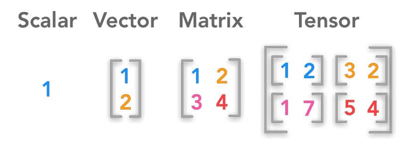
Scalar : 0차원 array (단일값)

Vector : 1차원 array

Matrix : 2차원 array

Tensor : 3차원(이상) array

1차원 array (벡터) 생성

np.array(iterable)

x = np.array([1,2,3])
y = np.array([2,4,15])

y # repr값

print(y) # str값

scalar

np.array(10)

type(x)

list는 원소타입이 제각각 다를 수 있다.

그러나, array는 모든 원소가 '한가지 타입' 이어야 함!

shape, size, ndim, dtype 그리고 len()

shape

numpy에서는 해당 array의 크기를 알 수 있다.

shape 을 확인함으로써 몇개의 데이터가 있는지, 몇 차원으로 존재하는지 등을 확인할 수 있다.

위에서 arr1.shape의 결과는 (5,) 으로써, 1차원의 데이터이며 총 5라는 크기를 갖고 있음을 알 수 있다.
arr4.shape의 결과는 (4,3) 으로써, 2차원의 데이터이며 4 * 3 크기를 갖고 있는 array 이다.

arr = np.array([1,2,3,4,5])
arr

arr.shape # tuple 타입이다.

(5,) <- 숫자의 개수는 차원

차원의 크기는 5

ndim : 차원 수

arr.ndim # 몇차원 데이터입니까?

ndim값 과 len(arr.shape) 은 같다!!!

size : 데이터 개수(스칼라 값의 개수)

arr.size

len(array) 배열의 개수

• array 도 iterable 하다!

len(arr)

dtype : data type

arr.dtype

dtype('int64') 정수 64bit (8byte)

5 개의 데이터가 있으므로 40 byte 사용중

arr2 = np.array([10, 3.14, 2, 0.12])
arr2

arr2.dtype

numpy에서 사용되는 자료형은 아래와 같다. (자료형 뒤에 붙는 숫자는 몇 비트 크기인지를 의미한다.)

부호가 있는 정수 int(8, 16, 32, 64)

부호가 없는 정수 uint(8 ,16, 32, 64)

실수 float(16, 32, 64, 128)

복소수 complex(64, 128, 256)

불리언 bool

문자열 string_

파이썬 오프젝트 object

유니코드 unicode_

2차원 array 생성

x = np.array([1, 2, 3, 4])
y = np.array([[2, 3, 4],[1, 2, 4]])

x

y

x.shape

y.shape

x.ndim

y.ndim

len(x)

len(y)

x.size

y.size

3차원

2 x 3 x 4

z = np.array([
[
[1, 2, 3, 4],
[5, 6, 7, 8],
[9, 10, 11, 12]
],
[
[101, 102, 103, 104],
[201, 202, 203, 204],
[301, 302, 303, 304]
]
])
z

z.shape

z.size

같은 스칼라 값이라도, '차원'이 다를 수 있다.

'차원 변환' 중요하다.

np.array(10) # scalar값 -- 0차원

np.array([10]) # 1차원

np.array([[10]]) # 2차원

np.array([[[10]]]) # 3차원

np.arange((3,10)) 2차원 배열 안됨 나중에 reshape로 변형할 수 있다

np.arange()

• range()와 사용법 유사

np.arange(10)

np.arange(1, 10)

np.arange(1, 10, 2)

np.arange(10, 0, -1)

np.arange(1, 10, dtype=np.int16)

astype(타입)

타입변환한 array 를 리턴 (원본 변화 없슴!)

d = np.arange(3, 10)
d # int64 타입

d.astype(np.float64)

d

reshape()

• ndarray의 형태, 차원을 바꾸기 위해 사용
• 머신러닝, 데이터 프로세싱에서 매우 자주 사용됨. (차원변환)

np.arange(12).reshape(2,6) # (12,) -> (2,6)

np.arange(12).reshape(2,4)

np.arange(12).reshape(3, 2, 2)

np.ones, np.zeros 로 array 생성

np.ones(5)

np.ones(6).reshape(2, 3)

np.ones((2,3), dtype=np.int16)

np.zeros((3,2,5), dtype=np.int8)

np.eye(5) # (5, 5) 단위 행렬

np.random 서브모듈

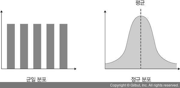
rand: 0부터 1사이의 균일 분포 [0, 1) uniform distribution

randn: 가우시안 표준 정규 분포

randint: 균일 분포의 정수 난수

np.random.rand(10)

np.random.rand(2,3)

np.random.randn(3,4,2)

np.random.randint(5) # 0 ~ 4 사이의 정수 난수

np.random.randint(1, 10) # 1 ~ 9 [1, 10)

np.random.randint(1, 100, (3, 5, 2))

np.unique()

np.unique([11, 11, 2, 2, 34, 34]) # unique 한 값으로 이루어진 array 리턴

인덱싱 index

• 파이썬 리스트와 동일한 개념으로 사용
• ,를 사용하여 각 차원의 인덱스에 접근 가능
• 인덱싱 할때마다 차원감소

x = np.arange(10)
x

x[0]

x[3] = 100
x

x = np.arange(10).reshape(2,5)
x

x[0] # (5,)

x[0][2]

x[0, 2] # <- 콤마로 인덱싱 가능! numpy 에선 후자의 방법을 추천!!!!

x

x[1, 4], x[1, -1], x[-1, -1]

Advanced indexing

• integer array indexing

x.shape

x[0]

x[[0]]

x[[1,0, 0, 0, 0, 0, 1, 0, 1, 1, 1, 1, 0]]

슬라이싱

• 리스트, 문자열 slicing과 동일한 개념으로 사용
• ,를 사용하여 각 차원 별로 슬라이싱 가능
• 슬라이싱은 차원 변화 없다

x = np.arange(10)
x

x[1:7]

x[1:]

x[:]

x[::2]

x[1::3]

x[::-1]

y = [[0, 1, 2, 3, 4],
[5, 6, 7, 8, 9],
[10, 11, 12, 13, 14]]
y

y[0:1]

y[1:3]

x = np.arange(15).reshape(3, 5)
x

x[:2][1:4]

x[:2, 1:4] # array는 차원별로 slicing 가능!!!!

---

ndarray shape (차원) 변경하기

차원변환은 데이터분석 과 인공지능에서 매우 빈번하게 발생되는 작업이니만큼 자유자재로 변환할수 있어야 하고, 머리속으로 내가 변환하는 데이터의 구조가 그려지도록 익숙해져야 합니다

사용 예) 이미지 데이터 벡터화 - 이미지는 기본적으로 2차원 혹은 3차원(RGB)이나 트레이닝을 위해 1차원으로 변경하여 사용 됨

ravel(), np.ravel()

• [ˈrævl]
• 다차원배열을 1차원으로 변경 (흔히 '펼친다'라고 말함)
• 'order' 파라미터
  • 'C' - row 우선 변경 , C style
  • 'F - column 우선 변경, Fortran style
• ravel() 은 np 안에 일반 함수로도 있고, 혹은 ndarray 의 멤버함수로서도 존재

x

x.ravel()

np.ravel(x)

np.ravel?

np.ravel(x, order = 'C') # row(행) 방향으로 펼쳐짐 차원축(axis) : (axis 0 부터 펼처짐)

np.ravel(x, order = 'F') # column(열) 방향으로 펼쳐짐 (axis -1 부터 펼처짐)

flatten()

• 다차원 배열을 1차원으로 변경
• ravel과의 차이점:
  • copy를 생성하여 변경함(즉 원본 데이터가 아닌 복사본을 반환)
  • ndarray 의 멤버함수로만 제공됨
• 'order' 파라미터
  • 'C' - row 우선 변경
  • 'F - column 우선 변경

y = np.arange(15).reshape(3,5)
y

y.flatten()

temp = x.ravel()
temp

temp[0] = 100
temp

x

temp2 = y.flatten() # 데이터의 '복사본'을 생성함
temp2

temp2[0] = 100
temp2

y # y는 바뀌지 않는다. (원본 데이터는 변화 없다!!!!)

reshape 함수

• array의 shape을 다른 차원으로 변경
• 주의할점은 reshape한 후의 결과의 전체 원소 개수와 이전 개수가 같아야 가능
• 사용 예) 이미지 데이터 벡터화 - 이미지는 기본적으로 2차원 혹은 3차원(RGB)이나 트레이닝을 위해 1차원으로 변경하여 사용 됨
• -1 값을 주어 나머지 차원을 유추하게 할수 있다

x2 = np.arange(36)
x2

x2.reshape(6,6)

x2.reshape(6, -1)

x2.reshape(6, -1, 2) # (6, 3, 2) 이런게 차원을 유추한다는 말이다.

차원 확장 / 제거

• 차원 확장/제거 하는 동작도 머신러닝에서 많이 사용된다.
• reshape() 로 차원 변환(확장/제거) 자유롭게 가능

차원 확장 : np.expand_dims()

• axis로 지정된 '차원을 추가'한다.

차원 자동 제거 : squeeze, np.squeeze()

• 차원 중 사이즈가 1인 것을 찾아 스칼라값으로 바꿔 해당 '차원을 제거'한다.

x3 = np.arange(6)
x3

x3.shape

x3 = x3.reshape(6, 1) # (6,) => (6,1) 로 차원 확장
x3

x3 = x3.reshape(6, 1, 1)
x3

x3 = x3.reshape((6,)) # 1차원으로 축소 (차원 제거)
x3

x3 = x3.reshape(1, 1, 1, 6)
x3

squeeze()

x3.squeeze()

x4 = np.arange(4).reshape((2, 1, 2))
x4

x4.squeeze()

x5 = np.arange(3)
x5

y5 = np.expand_dims(x5, 0) # 0번째 axis에 새로운 차원을 추가(삽입)한다.
y5

y5.shape

x6 = np.arange(4).reshape(2,2)
x6

마지막에 차원 추가

(2, 2) => (2, 2, 1)

y7 = np.expand_dims(x6, -1)
y7

a = np.array([2, 0, 1, 8])
a

1차원 벡터를 row vector 로 변환한다 라고 함.

a1 = a[np.newaxis, :] # (4,) => (1, 4)
a1

a1.shape

1차원 벡터를 coulmn vector로 변환한다 라고 함.

a2 = a[:, np.newaxis] # (4,) => (4,1)
a2

transpose, T, swapaxes

전치행렬 (transpose matrix) , 차원 축 바꾸기

a = np.arange(15).reshape(3, 5)
a

np.transpose(a) # (3, 5) => (5, 3)

a.T

np.swapaxes(a, 0, 1) # axis 0 과 axis 1을 바꾸기

기본연산, 기본함수

x = np.arange(15).reshape(3, 5)
y = np.arange(0, 150, 10).reshape(3, 5)
y2 = np.random.rand(15).reshape(3, 5)
y3 = np.arange(15).reshape(5, 3)

x

y

y2

y3

array간 연산

리스트의 경우

a = [10, 20, 30, 40]
b = 2
c = [100, 200, 300, 400]

a *2

a + c

array 연산은 리스트와 다르다!

기본적으로 '원소' 끼리 연산

x + y

x - y

array와 스칼라 값 연산도 가능

x + 10

단일값만 갖고 있는 객체와는 shape 와 관계없이, scalar 연산수행

x + [10]

x + [[10]]

x + np.array(10)

x + np.array([10])

x + np.array([10, 20]) # ValueError

에러이긴 하나... broadcast가 안돼서?

axis

"""
numpy 의 많은 함수들은 axis= 파라미터를 갖고 있습니다.
axis (축) 은 각 '차원' 을 의미합니다.
1차원 array 라면 각 차원에 대한 axis 값은 0 <- 1개 입니다.
2차원 array 라면 각 차원에 대한 axis 값은 0, 1 <- 2개 입니다.
3차원 array 라면 각 차원에 대한 axis 값은 0, 1, 2 <- 3개 입니다.

axis= 값을 명시하면 그 함수의 연산 은 해당 axis(축) 에 '따라서' 연산을 수행함

과연 '따라서' 의 의미가 무엇인지 실습을 통해 이해해봅시다
"""
None

x1 = np.arange(15)
x1

np.sum(x1)

np.sum(x1, axis=None)

x2 = x1.reshape(3,5)
x2

x2.shape

(행, 열)

(axis 0, axis 1)

np.sum(x2)

np.sum(x2, axis=0)

np.sum(x2, axis=1)

np.sum(x2, axis=-1)

np.sum(x2, axis=-2)

y = np.random.rand(15).reshape(3,5)
y

np.max(y)

np.argmax(y) # 최대값의 index

np.max(y, axis=0)

np.argmax(y, axis=0)

np.max(y, axis=1)

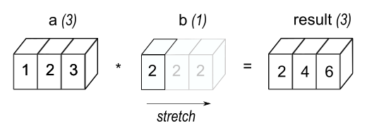
Broadcasting

브로드캐스팅

• (기본적으로는) Shape이 같은 두 ndarray에 대한 연산은 각 원소별로 진행
• 다른 Shape을 갖는 array 간 연산 의 경우 브로드 캐스팅(Shape을 맞춤) 후 진행

x = np.arange(15).reshape(3,5)
x

y = np.random.rand(15).reshape(3,5)
y

x+y

a = np.arange(12).reshape(4, 3)
b = np.arange(100, 103)

a

b # b.shape => (3,)

a + b

브로드캐스팅 Rule

• Rule 공식문서
• 뒷 차원에서 부터 비교하여 ①Shape이 같거나, ②차원 중 값이 1이 존재하면 broadcasting 가능
• 결과 차원은 둘중 큰 size 의 차원으로 확장 된다

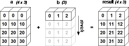
- 출처: https://www.tutorialspoint.com/numpy/images/array.jpg

''' 브로드캐스팅 가용한 경우
A : 256 x 256 x 3
B : 3
Result: 256 x 256 x 3 <-- 결과 차원은 둘중 큰 size의 차원으로 확장

A     : 8 x 1 x 6 x 1
B     :     7 x 1 x 5
Result: 8 x 7 x 6 x 5

'''

''' 브로드캐스팅 불가능한 경우
A : 3
B : 4

A     :     2 x 1
B     : 8 x 4 x 3

'''
None

c = np.arange(1000,1004)
c

a.shape, c.shape

Boolean Indexing

중요! 'Boolean indexing ' !

ndarry 인덱싱 시, bool 리스트를 전달하여 True인 경우만 필터링

for 사용하지 않고도 ndarray 에서 '조건'에 맞는 데이터만 추출 하는 기능

머신러닝 등에 있어서도 많이 사용

브로드캐스팅을 활용하여 ndarray로 부터 bool list 얻기

- 예) 짝수인 경우만 찾아보기

x = np.random.randint(1, 100, size = 10)
x

x % 2

x % 2 == 0

even_mask = x % 2 == 0
even_mask

위와 같이 bool 값으로 이루어진 array 를 Mask 라고도 한다

위 결과, mask 를 변수에 담아 보겠습니다

boolean mask로 인덱싱

x

x[even_mask]

Boolean Mask 로서 list, tuple 을 넣어주어도 필터 동작한다

x[[True, True, True, True, True, True, True, True, True, False]]

x[x % 2 == 0]

x[x > 30]

다중조건 사용하기

• 파이썬 논리 연산자인 and, or, not 키워드는 사용 불가
• & ← AND
• | ← OR

짝수 이면서 30보다 작은 숫자들

x[(x % 2 == 0) & (x < 50)]

astype()으로 변환

True, int(True), False, int(False)

(x > 50).astype(int)

(x > 50).astype(int).sum()

np.sum(x > 50)

temp = np.array(
[23.9, 24.4, 24.1, 25.4, 27.6, 29.7,
26.7, 25.1, 25.0, 22.7, 21.9, 23.6,
24.9, 25.9, 23.8, 24.7, 25.6, 26.9,
28.6, 28.0, 25.1, 26.7, 28.1, 26.5,
26.3, 25.9, 28.4, 26.1, 27.5, 28.1, 25.8])

"""
평균기온이 25도를 넘는 날수는 총 21일
평균기온이 25를 넘는 날의 평균 기온은 약 26.8도
"""
None

np.sum(temp > 25.0)

temp[temp > 25]

print("%0.2f", sum(temp[temp > 25]) / len(temp[temp > 25]))

np.mean(temp[temp > 25])

np.average(temp[temp > 25])