Edges
Edge Detection
Line segments where the image brightness changes sharply (or has discontinuities)
2D image를 curve의 집합으로 convert
- scene의 눈에 띄는(salient) feature 추출
- pixel들보다 compact
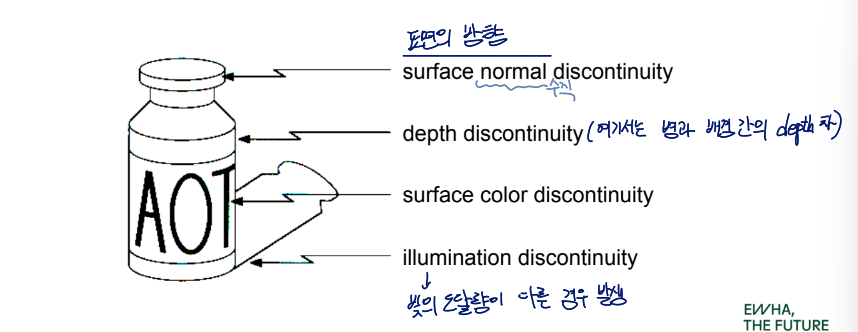
Origin of Edges
Edges는 다양한 요소로 인해 발생함
- surface normal discontinuity
불연속적인 표면 방향
여기서 normal은 수직이라는 뜻
- depth discontinuity
- surface color discontinuity
- illumination discontinuity
빛의 도달량이 다른 경우
Edge Types
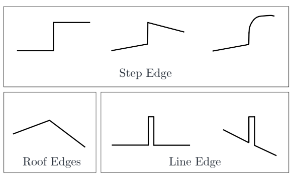
근데 그렇게 크게 중요하진 않음
Ideal Edge Operator
edge operator는
- Edge Magnitude
- Edge Orientation
orientation : 방향
- High Detection Rate and Good Localization
detection: edge를 검출 잘하는지, locatlization: edge를 잘 그렸는지
을 produce해야 함
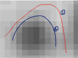
이 경우, 알고리즘 2가 1보다 edge localization을 잘함
Gradient
Gradient equation
▽f=[∂x∂f,∂y∂f]
intensity가 가장 급격하게 변화하는 방향을 표현함
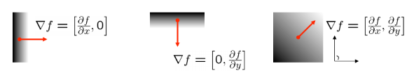
edge의 기울기와는 수직
Gradient direction
θ=tan−1(∂y∂f/∂x∂f)
edge strength는 gradient magnitude로 주어짐
∥▽f∥=(∂x∂f)2+(∂y∂f)2
Theory of Edge Detection
Ideal edge
continuous space에서의 ideal edge

- L(x,y)=xsin(θ)−ycos(θ)+ρ=0
edge가 선으로 정의됨
- B1:L(x,y)<0
- B2:L(x,y)>0
Unit step function
u(t)=⎩⎪⎪⎨⎪⎪⎧11/20for t>0for t=0for t<0u(t)=∫−∞tδ(s)ds
Image intensity (brightness)
I(x,y)=B1+(B2−B1)u(xsinθ−ycosθ+ρ)
- u()=0→B1
- u()=21→중간값
- u()=1→B2
Partial derivates (gradients)
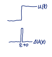
- ∂x∂I=+sinθ(B2−B1)δ(xsinθ−ycosθ+ρ)
- ∂y∂I=−cosθ(B2−B1)δ(xsinθ−ycosθ+ρ)
δ(): dirac delta function
Squared gradient
s(x,y)=(∂x∂I)2+(∂y∂I)2=[(B2−B1)δ(xsinθ−ycosθ+ρ)]2
- Edge magnitude: s(x,y)
- Edge orientation: arctan∂y∂I/∂x∂I
edge에 수직인 방향
Laplacian
▽2I=∂x2∂2I+∂y2∂2I=(B2−B1)δ′(xsinθ−ycosθ+ρ)
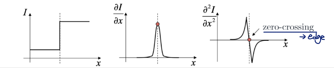
zero-crossing하는 부분이 edge
Edge Detection in Image
Edge Detection in Image
- How would you go about detecting edges (i.e., discontinuities) in an image?
- 미분 실행 : discontinuities는 큰 미분값을 가짐
- How do you differntiate a discrete image (or any other discrete signal)?
Finite Differences
이미지는 discrete하기 때문에 다음과 같은 방식으로 기울기를 구함
-
Definition of a derivate using forward difference
f′(x)=h→0limhf(x+h)−f(x)
- h=1의 경우 convolution kernel
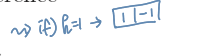
-
Alternative: central difference 사용
f′(x)=h→0limhf(x+0.5h)−f(x−0.5h)
0.5h : offset
-
For discrete signals: Remove limit and set h=2
f′(x)=2f(x+1)−f(x−1)
∵ discrete에서는 offset의 최솟값=1
Discrete Edge Filters
2D filter가 1D보다 robust함
Roberts (1965)
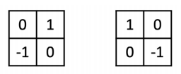
잘 작동은 못하지만 역사적으로 의미있는 커널
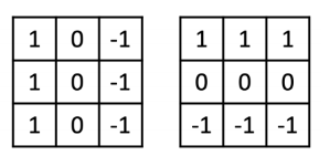
Prewitt (1970)
Sobel (1970)
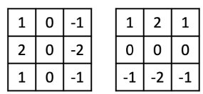
많이 사용됨
가까운 픽셀에 값을 더 치중함으로써 noise에 강해짐
Effect of Noise
differentiation은 noise에 매우 민감함
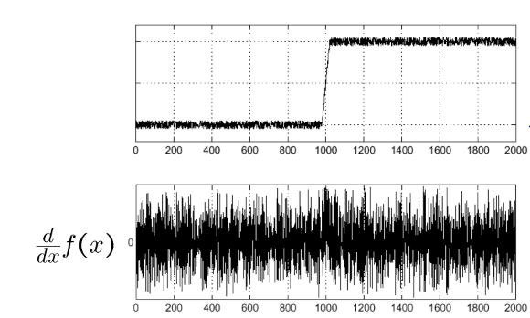
noise로 인해 edge를 찾기 어려워짐
→ 노이즈를 제거해야 더 나은 edge detect를 수행할 수
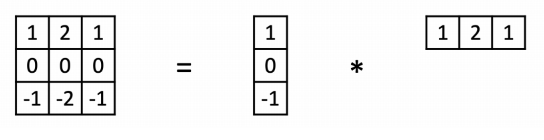
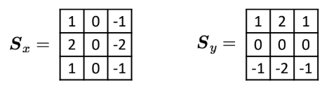
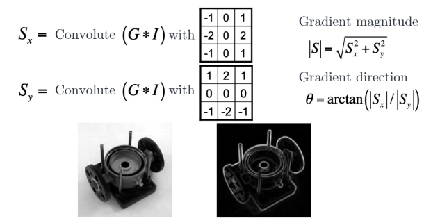
Sobel Filter
sobel filter는 smoothing effect까지 주도록 만들어진 filter
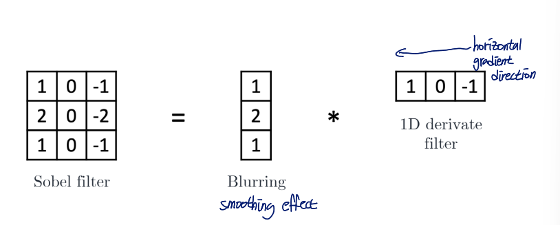
- horizontal sobel filter
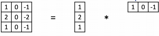
- vertical sobel filter
Sobel Filter Example
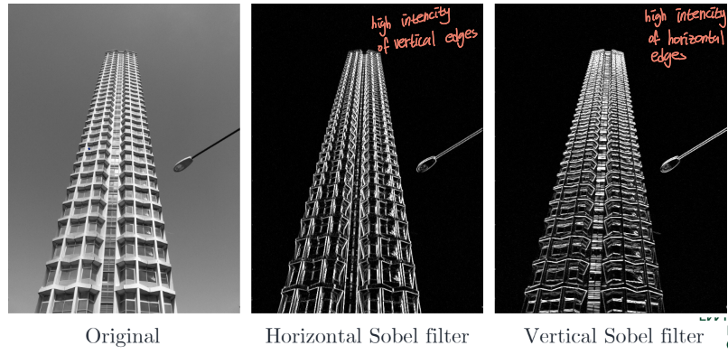
간단하게 생각하면 이름과 수직 방향의 edge들이 집중적으로 detect됨
Discrete Edge Filters
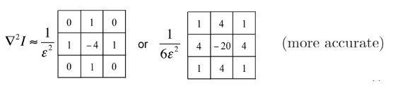
Laplacian을 사용해 edge detection을 하고자 함
Second order partial derivatives
- ∂x2∂2I≈ε21(Ii−1,j−2Ii,j+Ii+1,j)
- ∂y2∂2I≈ε21(Ii,j−1−2Ii,j+Ii,j+1)
Laplacian
▽2I=∂x2∂2I+∂y2∂2I
- convolution masks
Comparing Edge Operators
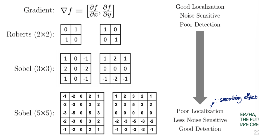
필터가 커질수록
- localization은 못하지만
- noise에 있어서 robust하고
- detection 수행을 잘 함
노이즈를 제거함으로써
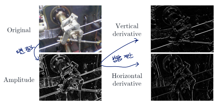
Computing Image Gradients
- derivative filters 선택
- 이미지와 convolusion 통해 기울기 구하기
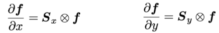
- image gradient를 form하고 direction과 amplitude 계산
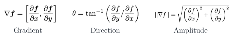
Image Gradient Example
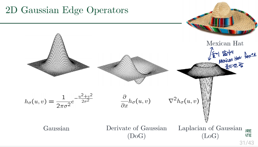
Derivative of Gaussian (DoG) Filter
smoothing을 먼저 하고 기울기를 구함으로써 노이즈에 robust해지기 위한 방법
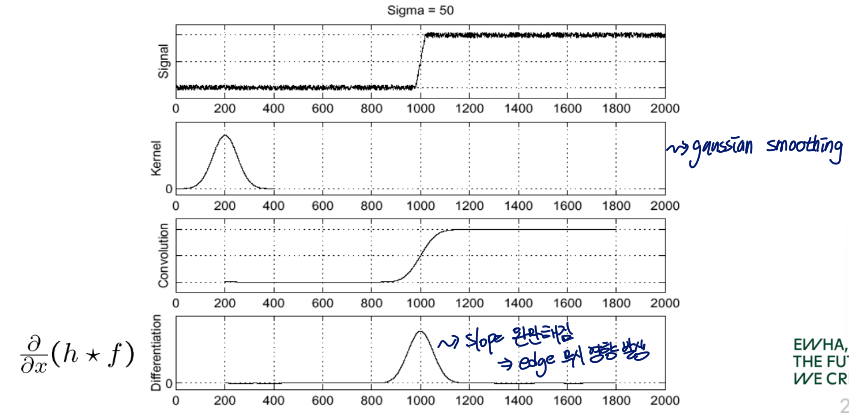
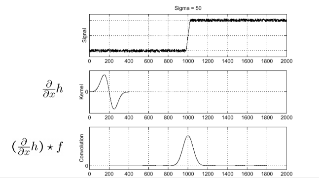
kernel의 기울기를 먼저 구하고 f와 convolve
→ 더 빠르게 계산 가능
∂x∂(h⋆f)=(∂x∂h)⋆f
one operation이 save됨
Laplacian of Gaussian (LoG) Filter
∂x2∂2(h⋆f)=(∂x2∂2h)⋆f
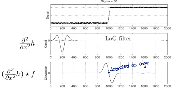
edge는 zero-crossings of bottom graph를 통해 찾을 수 있음
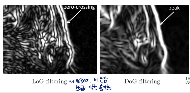
LoG vs. DoG Filtering
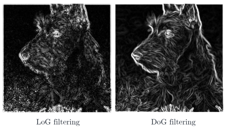
zero crossings가 localizing edges에 더 정확하지만 convenient하지 음
2D Gaussian Edge Operators
Canny Edge Detector
Canny Edge Detector
- 2D Gaussian을 통해 smooth image: G∗I

- Find the gradient magnitude and direction for each pixel
- non-maximum suppression(NMS) 실행
sharp edges를 얻기
∵ 이상적인 edge: 선
- double thresholding and Edge tracking by hysteresis
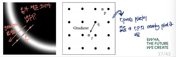
Non-Maximum Suppression(NMS)
pixel이 gradient direction에서 local maximum인지 확인
- edge strength of the current pixel (q)를 이웃 픽셀들과 비교
- q의 strength가 가장 큰 경우 보존, 아닌 경우 suppress(i.e., set to 0)
- requires checking interpolated pixels p and r
Thresholding
Standard Thresholding
E(x,y)={10if ∥(x,y)∥>T for some threshold Totherwise
strong edges만 고를 수 있지만 continuity를 보장하지 않음
Hysteresis based Thresholding
2개의 threshold 사용
∥▽f(x,y)∥≥t1definitely an edget0≥∥▽f(x,y)∥<t1maybe an edge, depends on context∥▽f(x,y)∥<t1definitely not an edge
maybe edges는 strong edge의 근처에 있으면 edge로 판별
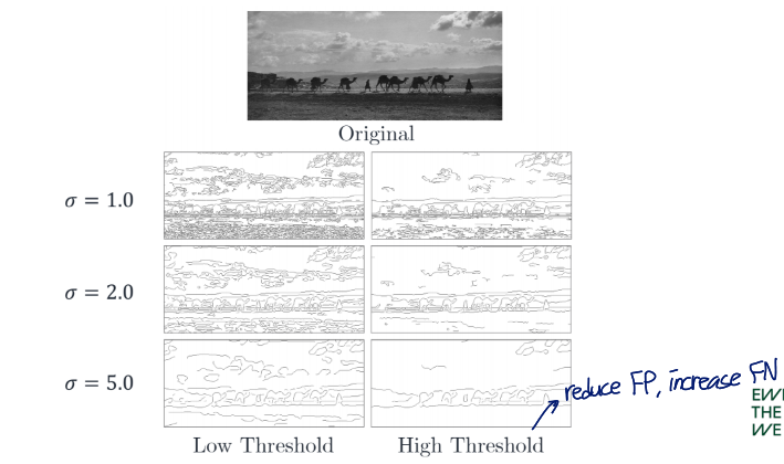
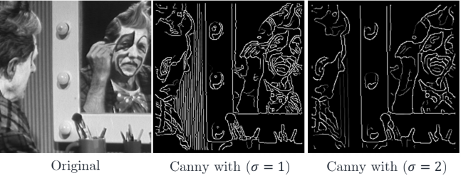
Paramters
parameter setting is critical
standard deviation of Gaussian filter : σ
desired behavior에 따라 선택
- Large σ : large-scale edges 탐지
detail을 놓칠 수 있음
- Small σ : fine features 탐지
two threshold values