How to Represent Signals?
Taylor series는 polynomials를 사용하여 모든 함수를 표현할 수 있음f ( x ) = f ( a ) + f ′ ( a ) ( x − a ) + f ′ ′ ( a ) 2 ! ( x − a ) 2 + f ′ ′ ′ ( a ) 3 ! ( x − a ) 3 + . . . f(x) = f(a)+f'(a)(x-a)+\frac{f''(a)}{2!}(x-a)^2 + \frac{f'''(a)}{3!}(x-a)^3+... f ( x ) = f ( a ) + f ′ ( a ) ( x − a ) + 2 ! f ′ ′ ( a ) ( x − a ) 2 + 3 ! f ′ ′ ′ ( a ) ( x − a ) 3 + . . .
그러나
polynomials are not the best
unstable and not very physically meaningfulcomputational cost가 높음
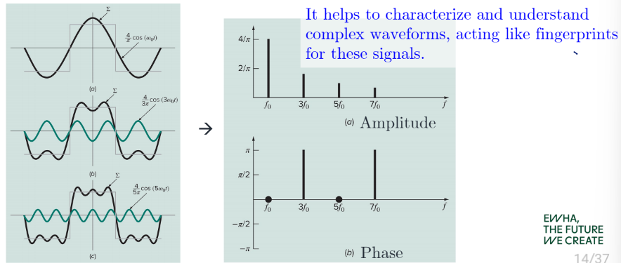
easier to talk about signals in terms of its frequencies (how fast/often signals change, etc)
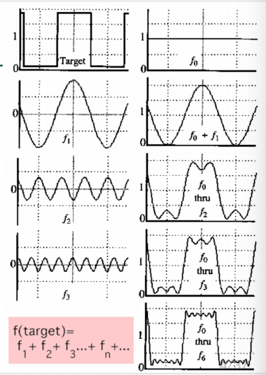
Fourier Analysis
복잡한 time-series의 함수가 간단한 sinusoidal functions들의 합으로 표현될 수 있다는 전제에 기반
Sinusoidal function: A general term for periodic functions주기 함수의 일반적 용어라는 뜻
Curve Fitting with Sinusoidal Functions
Periodic function
f ( t ) = f ( t + T ) w h e r e T : p e r i o d f(t) = f(t+T)\quad\space where \quad T:period f ( t ) = f ( t + T ) w h e r e T : p e r i o d
A common example: Sinusoidal function
sine or cosine function
주기 : π / 2 \pi/2 π / 2
여기서는 cosine을 basis for explanations로 사용할 것임
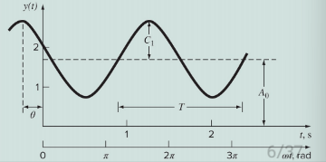
Sinusoidal function
f ( t ) = A 0 + C 1 cos ( w 0 t + θ ) f(t) = A_0 + C_1\cos(w_0t+\theta) f ( t ) = A 0 + C 1 cos ( w 0 t + θ )
Mean vlaue A 0 A_0 A 0
Amplitude C 1 C_1 C 1
Angular frequency w 0 w_0 w 0
relationship between ordinary frequency and period T w 0 = 2 π f = 2 π T \space w_0 = 2\pi f = \frac{2\pi}{T} w 0 = 2 π f = T 2 π
Phase angle θ \theta θ
phase angle이 들어가면 곡선을 fitting하는 과정이 좀 복잡해짐
Trigonometric identity cos ( x + y ) = cos x cos y − sin x sin y \cos(x+y) = \cos{x}\cos{y} - \sin{x}\sin{y} cos ( x + y ) = cos x cos y − sin x sin y
Then,
C 1 cos ( w 0 t + θ ) = C 1 [ cos ( w 0 t ) cos ( θ ) − sin ( w 0 t ) sin ( θ ) ] C_1\cos{(w_0t+\theta)} = C_1[\cos{(w_0t)}\cos{(\theta)} - \sin{(w_0t)}\sin{(\theta)}] C 1 cos ( w 0 t + θ ) = C 1 [ cos ( w 0 t ) cos ( θ ) − sin ( w 0 t ) sin ( θ ) ] → f ( t ) = A 0 + A 1 cos ( w 0 t ) + B 1 sin ( w 0 t ) \rightarrow f(t) = A_0+A_1\cos{(w_0t)} + B_1\sin{(w_0t)} → f ( t ) = A 0 + A 1 cos ( w 0 t ) + B 1 sin ( w 0 t ) \quad C 1 = A 1 2 + B 1 2 a n d θ = a r c t a n ( − B 1 / A 1 ) C_1 = \sqrt{A_1^2 + B_1^2}\quad and \quad \theta = arctan(-B_1/A_1) C 1 = A 1 2 + B 1 2 a n d θ = a r c t a n ( − B 1 / A 1 ) cos ( θ ) = C 1 A 1 \quad\space\cos(\theta) = \frac{C_1}{A_1} cos ( θ ) = A 1 C 1 sin ( θ ) = − C 1 B 1 \sin(\theta) = -\frac{C_1}{B_1} sin ( θ ) = − B 1 C 1 tan ( θ ) = − A 1 B 1 \tan(\theta) = -\frac{A_1}{B_1} tan ( θ ) = − B 1 A 1
Another example of a general linear regression model → can apply the least squares methody = β 0 ⋅ f 0 ( x 1 , x 2 , . . . , x p ) + β 1 ⋅ f 1 ( x 1 , x 2 , . . . , x p ) + . . . + β m ⋅ f m ( x 1 , x 2 , . . . , x p ) + ϵ y = \beta_0\cdot f_0(x1,x_2,...,x_p) + \beta_1\cdot f_1(x_1,x_2,...,x_p) + ... + \beta_m\cdot f_m(x_1,x_2,...,x_p)+\epsilon y = β 0 ⋅ f 0 ( x 1 , x 2 , . . . , x p ) + β 1 ⋅ f 1 ( x 1 , x 2 , . . . , x p ) + . . . + β m ⋅ f m ( x 1 , x 2 , . . . , x p ) + ϵ
Sum of squared errors (SSE)
S S E = ∑ N i = 1 { y i − [ A 0 + A 1 cos ( w 0 t ) + B 1 sin ( w 0 t ) ] } 2 SS_E = \underset{i=1}{\overset{N}{\sum}}\{y_i - [A_0 + A_1\cos(w_0t) + B_1\sin(w_0t)]\}^2 S S E = i = 1 ∑ N { y i − [ A 0 + A 1 cos ( w 0 t ) + B 1 sin ( w 0 t ) ] } 2 그냥 real value에 estimated value를 뻰 값을 제곱한 거임
에러를 계산하는 거니까 당연히 작은 값이 나오도록 해야 됨
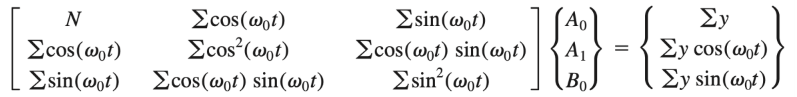
Normal equation
△ t \bigtriangleup t △ t T = ( N − 1 ) △ t T=(N-1)\bigtriangleup t T = ( N − 1 ) △ t ( A 0 , A 1 , B 1 ) (A_0,A_1,B_1) ( A 0 , A 1 , B 1 )
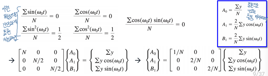
따라서f ( t ) = A 0 + A 1 cos ( w 0 t ) + B 1 sin ( w 0 t ) f(t) = A_0+A_1\cos{(w_0t)} + B_1\sin{(w_0t)} f ( t ) = A 0 + A 1 cos ( w 0 t ) + B 1 sin ( w 0 t )
A 0 = ∑ y N A_0 = \frac{\sum y}{N} A 0 = N ∑ y A 1 = 2 N ∑ y cos ( w 0 t ) A_1 = \frac{2}{N}\sum y\cos(w_0t) A 1 = N 2 ∑ y cos ( w 0 t ) B 1 = 2 N ∑ y sin ( w 0 t ) B_1 = \frac{2}{N}\sum y\sin(w_0t) B 1 = N 2 ∑ y sin ( w 0 t )
General model
더 자세히 표현할 경우f ( t ) = A 0 + A 1 cos ( w 0 t ) + B 1 sin ( w 0 t ) + A 2 cos ( 2 w 0 t ) + B 2 ( 2 w 0 t ) + . . . + A m cos ( m w 0 t ) + B m sin ( m w 0 t ) f(t) = A_0 + A_1\cos(w_0t)+B_1\sin(w_0t)+A_2\cos(2w_0t)+B_2(2w_0t)+...+A_m\cos(mw_0t)+B_m\sin(mw_0t) f ( t ) = A 0 + A 1 cos ( w 0 t ) + B 1 sin ( w 0 t ) + A 2 cos ( 2 w 0 t ) + B 2 ( 2 w 0 t ) + . . . + A m cos ( m w 0 t ) + B m sin ( m w 0 t )
A 0 = ∑ y N A_0 = \frac{\sum y}{N} A 0 = N ∑ y A j = 2 N ∑ y cos ( j w 0 t ) A_j = \frac{2}{N}\sum y\cos(jw_0t) A j = N 2 ∑ y cos ( j w 0 t ) B j = 2 N ∑ y sin ( j w 0 t ) B_j = \frac{2}{N}\sum y\sin(jw_0t) B j = N 2 ∑ y sin ( j w 0 t ) j = 1 , 2 , . . . , m j=1,2,...,m j = 1 , 2 , . . . , m
Continuous Fourier Series
fourier는 모든 주기 함수는 infinite series of sinusoidal functions로 표현될 수 있다는 것을 증명함
function with period T에 따라 Fourier series는 다음과 같이 표현됨f ( t ) = a 0 + a 1 cos ( w 0 t ) + b 1 sin ( w 0 t ) + a 2 cos ( 2 w 0 t ) + b 2 sin ( 2 w 0 t ) + . . . f(t) = a_0 + a_1\cos(w_0t)+b_1\sin(w_0t)+a_2\cos(2w_0t)+b_2\sin(2w_0t)+... f ( t ) = a 0 + a 1 cos ( w 0 t ) + b 1 sin ( w 0 t ) + a 2 cos ( 2 w 0 t ) + b 2 sin ( 2 w 0 t ) + . . . = a 0 + ∑ ∞ k = 1 [ a k cos ( k w 0 t ) + b k sin ( k w 0 t ) ] \quad\quad= a_0 + \underset{k=1}{\overset{\infty}{\sum}}[a_k\cos(kw_0t)+b_k\sin(kw_0t)] = a 0 + k = 1 ∑ ∞ [ a k cos ( k w 0 t ) + b k sin ( k w 0 t ) ] w h e r e a k = 2 T ∫ 0 T f ( t ) cos ( k w 0 t ) d t b k = 2 T ∫ 0 T f ( t ) sin ( k w 0 t ) d t a 0 = 1 T ∫ 0 T f ( t ) d t \quad\quad where \quad a_k = \frac{2}{T}\int_0^T f(t)\cos(kw_0t)dt\\ \quad\quad\quad\quad\quad\space\space\space b_k=\frac{2}{T}\int_0^T f(t)\sin(kw_0t)dt\\ \quad\quad\quad \quad \quad \space \space \space a_0 = \frac{1}{T}\int_0^T f(t)dt w h e r e a k = T 2 ∫ 0 T f ( t ) cos ( k w 0 t ) d t b k = T 2 ∫ 0 T f ( t ) sin ( k w 0 t ) d t a 0 = T 1 ∫ 0 T f ( t ) d t
w 0 w_0 w 0 2 w 0 , 3 w 0 , . . . 2w_0,3w_0,... 2 w 0 , 3 w 0 , . . .
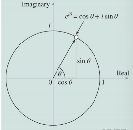
e ± i x = cos x ± i sin x e^{\pm ix} = \cos x \pm i\sin x e ± i x = cos x ± i sin x
이 공식을 사용해서 Fourier series를 더 compact하게 표현할 수 있음
f ( t ) = ∑ ∞ k = − ∞ c ~ k e i k w 0 t f(t) = \underset{k=-\infty}{\overset{\infty}{\sum}}\tilde{c}_ke^{ikw_0t} f ( t ) = k = − ∞ ∑ ∞ c ~ k e i k w 0 t c ~ k = 1 T ∫ − T 2 T 2 f ( t ) e i k w 0 t d t \tilde{c}_k = \frac{1}{T}\int_{-\frac{T}{2}}^{\frac{T}{2}}f(t)e^{ikw_0t}dt c ~ k = T 1 ∫ − 2 T 2 T f ( t ) e i k w 0 t d t
Euler's formula에서 얻은 정보
cos x = e i x + e − i x 2 \cos x = \frac{e^{ix}+e^{-ix}}{2} cos x = 2 e i x + e − i x sin x = e i x − e − i x 2 i \sin x = \frac{e^{ix}-e^{-ix}}{2i} sin x = 2 i e i x − e − i x
Frequency and Time Domains
위에서의 Fourier analysis는 시간 domain으로 제한이 되어 있음
예시f ( t ) = C 1 cos ( t + π 2 ) f(t) = C_1\cos(t+\frac{\pi}{2}) f ( t ) = C 1 cos ( t + 2 π )
(b) : projection of the curve onto the time plane
(c) : projection of the curve onto the frequency plane
(d) : projection of the curve onto the phase angle plane
Fourier series와 같은 complex cases의 경우에는
reality에는 non-repetitive(non-periodic)한 waveforms도 많음
Fourier Integral
transition from periodic to non-periodic functions can be achieved by letting the period T approach infinityT를 무한대로 설정하면 주기함수를 non-periodic 함수로 변환할 수 있음
T가 infinite가 되면 function은 다시 반복하지 않게 됨 → 주기가 없어짐
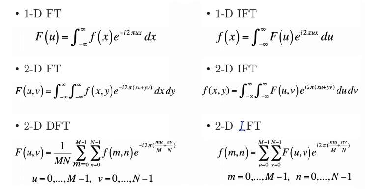
{ f ( t ) = 1 2 π ∫ − ∞ ∞ F ( i w 0 ) e i w 0 t d w 0 Inverse Fourier Transform (IFT) F ( i w 0 ) = ∫ − ∞ ∞ f ( t ) e − i w 0 t d t Fourier Transform (FT) \begin{cases} f(t) = \frac{1}{2\pi}\int_{-\infty}^{\infty} F(iw_0)e^{iw_0t}dw_0 & \text{Inverse Fourier Transform (IFT)}\\ F(iw_0) = \int_{-\infty}^{\infty}f(t)e^{-iw_0t}dt & \text{Fourier Transform (FT)} \end{cases} { f ( t ) = 2 π 1 ∫ − ∞ ∞ F ( i w 0 ) e i w 0 t d w 0 F ( i w 0 ) = ∫ − ∞ ∞ f ( t ) e − i w 0 t d t Inverse Fourier Transform (IFT) Fourier Transform (FT) 밑의 식을 위로 변환하면 IFT, 위의 식을 아래로 변환하면 FT라는 뜻임
IFT, FT에 따른 결과는 이런 식으로 됨↓
복기 : 주기가 있는 경우{ f ( t ) = ∑ ∞ k = − ∞ c ~ k e i k w 0 t Inverse Fourier Transform (IFT) c ~ k = 1 T ∫ − T / 2 T / 2 f ( t ) e − k w 0 t d t Fourier Transform (FT) \begin{cases}f(t) = \underset{k=-\infty}{\overset{\infty}{\sum}}\tilde{c}_k e^{ikw_0t} & \text{Inverse Fourier Transform (IFT)}\\ \tilde{c}_k = \frac{1}{T}\int_{-T/2}^{T/2}f(t)e^{-kw_0t}dt & \text{Fourier Transform (FT)}\end{cases} ⎩ ⎪ ⎪ ⎨ ⎪ ⎪ ⎧ f ( t ) = k = − ∞ ∑ ∞ c ~ k e i k w 0 t c ~ k = T 1 ∫ − T / 2 T / 2 f ( t ) e − k w 0 t d t Inverse Fourier Transform (IFT) Fourier Transform (FT)
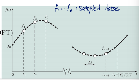
일반적으로, 데이터는 discrete values로 수집됨△ T / n \bigtriangleup T/n △ T / n
F k = ∑ N − 1 n = 0 f n e i k w 0 n for k=0 to N-1 F_k = \underset{n=0}{\overset{N-1}{\sum}}f_ne^{ikw_0n}\quad \quad\quad\text{for k=0 to N-1} F k = n = 0 ∑ N − 1 f n e i k w 0 n for k=0 to N-1 적분을 급수함수로 변경한 임
f n = 1 N ∑ N − 1 k = 0 F k e i k w 0 n for n=0 to N-1 f_n = \frac{1}{N}\underset{k=0}{\overset{N-1}{\sum}}F_ke^{ikw_0n} \quad\quad\text{for n=0 to N-1} f n = N 1 k = 0 ∑ N − 1 F k e i k w 0 n for n=0 to N-1
DFT는 n 2 n^2 n 2
FFT는 DFT를 더 효율적으로 계산할 수 있도록 만들어진 알고리즘F k = ∑ N − 1 n = 0 f n e − i k w 0 n F_k = \underset{n=0}{\overset{N-1}{\sum}}f_ne^{-ikw_0n} F k = n = 0 ∑ N − 1 f n e − i k w 0 n
이전 계산 결과를 재사용 함으로써 계산량을 줄임in particular, it leverages the periodicity and symmetry of trigonometric functions
O ( n 2 ) → O ( n log n ) O(n^2)\rightarrow O(n\log n) O ( n 2 ) → O ( n log n )
근데 요즘은 DFT, FFT 구분 잘 안한다고 함
Power Spectrum
electrical engineering에서 power는 일반적으로 proportional to the square of the voltage or current함
this concept is extended to Fourier analysis, where power is calculated as the sum of the squares (or the integral) of the Fourier coefficietns
P k = ∣ c ~ k ∣ 2 or P ( w ) = ∣ F ( w ) ∣ 2 P_k = \lvert\tilde{c}_k\rvert^2 \quad \text{or} \quad P(w)=\lvert F(w)\rvert^2 P k = ∣ c ~ k ∣ 2 or P ( w ) = ∣ F ( w ) ∣ 2
Other Frequency Spectrums
여기에 나오는 식들에서 R: realvalue(실수부), I: imaginal value(허수부)
Complex spectrum
F ( u , v ) = R ( u , v ) + i I ( u , v ) F(u,v) = R(u,v)+iI(u,v) F ( u , v ) = R ( u , v ) + i I ( u , v )
Magnitude spectrum
∣ F ( u , v ) ∣ = R 2 ( u , v ) + I 2 ( u , v ) \lvert F(u,v)\rvert = \sqrt{R^2(u,v) + I^2(u,v)} ∣ F ( u , v ) ∣ = R 2 ( u , v ) + I 2 ( u , v )
Phase spectrum
ϕ ( u , v ) = tan − 1 ( I ( u , v ) / R ( u , v ) ) \phi (u,v) = \tan^{-1}(I(u,v)/R(u,v)) ϕ ( u , v ) = tan − 1 ( I ( u , v ) / R ( u , v ) )
Power spectrum
일반적으로 사용P ( u , v ) = ∣ F ( u , v ) ∣ 2 = R 2 ( u , v ) + I 2 ( u , v ) P(u,v) = \lvert F(u,v)\rvert^2 = R^2(u,v) + I^2(u,v) P ( u , v ) = ∣ F ( u , v ) ∣ 2 = R 2 ( u , v ) + I 2 ( u , v )
Cosine function with frequency
f ( x ) = cos ( w 0 x ) F ( u ) = π 2 ⋅ ( δ ( u + w 0 ) + δ ( u − w 0 ) ) f(x) = \cos(w_0x) \quad\quad F(u) = \sqrt{\frac{\pi}{2}}\cdot (\delta(u+w_0)+\delta(u-w_0)) f ( x ) = cos ( w 0 x ) F ( u ) = 2 π ⋅ ( δ ( u + w 0 ) + δ ( u − w 0 ) )
e.g. w 0 = 3 w_0 = 3 w 0 = 3
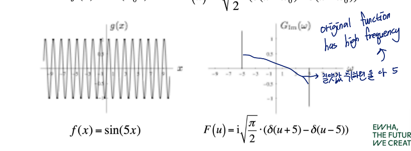
Sine function with frequency
f ( x ) = sin ( w 0 x ) F ( u ) = i π 2 ⋅ ( δ ( u + w 0 ) − δ ( u − w 0 ) ) f(x) = \sin(w_0x) \quad\quad F(u) = i\sqrt{\frac{\pi}{2}}\cdot (\delta(u+w_0)-\delta(u-w_0)) f ( x ) = sin ( w 0 x ) F ( u ) = i 2 π ⋅ ( δ ( u + w 0 ) − δ ( u − w 0 ) )
e.g. w 0 = 5 w_0 = 5 w 0 = 5
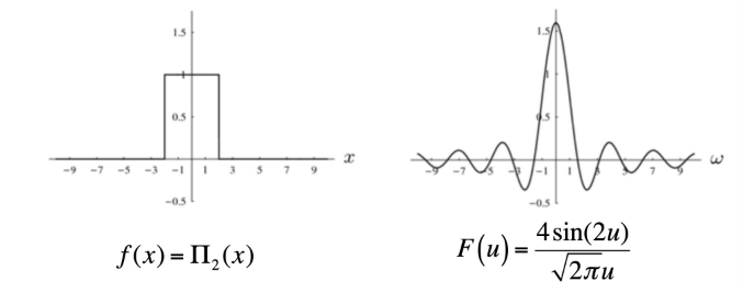
Rectangular pulse
f ( x ) = Π b ( x ) = { 1 for |x| ≤ b 0 otherwise F ( u ) = π 2 ( δ ( u + w 0 ) + δ ( u − w 0 ) ) f(x)=\Pi_b(x) = \begin{cases} 1 & \text{for |x|}\leq b \\ 0 & \text{otherwise} \end{cases} \quad\quad F(u) = \sqrt{\frac{\pi}{2}}(\delta(u+w_0)+\delta(u-w_0)) f ( x ) = Π b ( x ) = { 1 0 for |x| ≤ b otherwise F ( u ) = 2 π ( δ ( u + w 0 ) + δ ( u − w 0 ) )
e.g. b = 2 b=2 b = 2
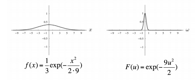
Gaussian function
f ( x ) = 1 σ exp ( − x 2 2 σ 2 ) F ( u ) = exp ( − σ 2 u 2 2 ) f(x) = \frac{1}{\sigma}\exp(-\frac{x^2}{2\sigma^2}) \quad\quad F(u)=\exp(-\frac{\sigma^2u^2}{2}) f ( x ) = σ 1 exp ( − 2 σ 2 x 2 ) F ( u ) = exp ( − 2 σ 2 u 2 )
e.g. σ = 3 \sigma=3 σ = 3
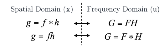
Convolution in spatial domain ⟷ Multiplication in frequency domain \text{Convolution in spatial domain} \longleftrightarrow \text{Multiplication in frequency domain} Convolution in spatial domain ⟷ Multiplication in frequency domain
따라서, g ( x ) g(x) g ( x )
각각 f, h에 FT 실행
두 값 곱하기
곱한 값 IFT 취하기
convolution 연산량이 많은 경우 이렇게 계산하는 것을 통해 연산량을 줄일 수 있음
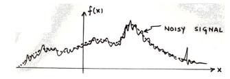
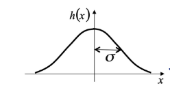
Example use: Smoothing/Blurring
f ( x ) f(x) f ( x ) g ( x ) = f ( x ) ∗ h ( x ) \quad \quad g(x) = f(x)*h(x) g ( x ) = f ( x ) ∗ h ( x ) 가우시안 커널을 사용할 것임h ( x ) = 1 2 π σ exp [ − 1 2 ( 2 π u ) 2 σ 2 ] \quad\quad h(x)=\frac{1}{\sqrt{2\pi}\sigma}\exp\big[-\frac{1}{2}(2\pi u)^2\sigma^2\big] h ( x ) = 2 π σ 1 exp [ − 2 1 ( 2 π u ) 2 σ 2 ]
Then,
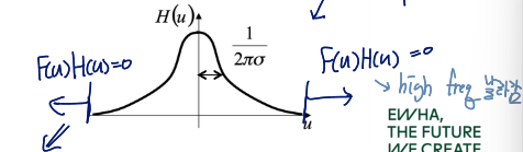
H ( u ) = exp ⌊ − 1 2 ( 2 π u ) 2 σ 2 ⌋ \quad\quad H(u) = \exp\lfloor -\frac{1}{2}(2\pi u)^2\sigma^2\rfloor H ( u ) = exp ⌊ − 2 1 ( 2 π u ) 2 σ 2 ⌋ G ( u ) = F ( u ) H ( u ) \quad\quad G(u) = F(u)H(u) G ( u ) = F ( u ) H ( u )
H ( u ) H(u) H ( u ) F ( u ) F(u) F ( u ) Low-pass Filter
별 다른 거 없음..
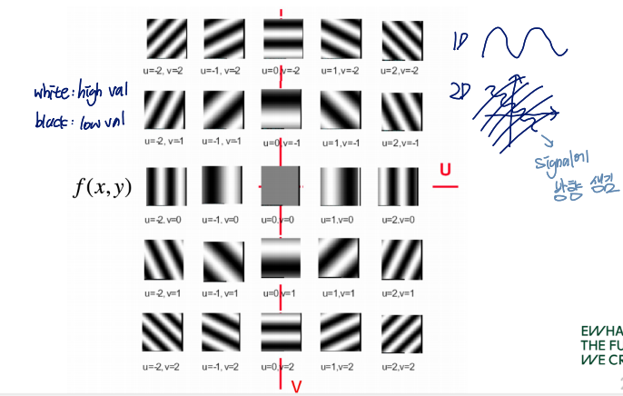
2D의 경우, 1D에 없었던 방향이 생김
spatial function f ( x , y ) f(x,y) f ( x , y )
f ( x , y ) = ∫ − ∞ ∞ ∫ − ∞ ∞ F ( u , v ) e i 2 π ( x u + y v ) d u d v f(x,y) = \int_{-\infty}^{\infty}\int_{-\infty}^{\infty}F(u,v)e^{i2\pi(xu+yv)}dudv f ( x , y ) = ∫ − ∞ ∞ ∫ − ∞ ∞ F ( u , v ) e i 2 π ( x u + y v ) d u d v
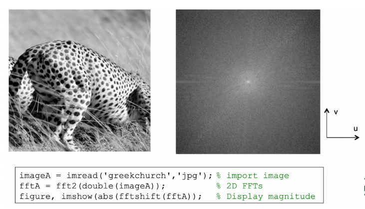
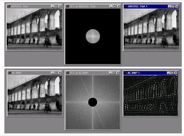
Image Processing in the Fourier Domain
RGB의 경우는 각각 chanel에 적용 후 평균을 구하는 식으로 진행함
Convolution is Mulfiplication in Fourier Domain
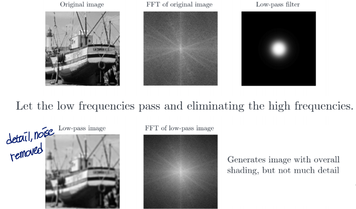
Low-Pass Filtering
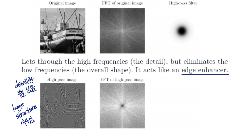
High-Pass Filtering
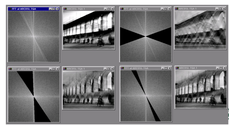
Fun with Fourier Spectra