K-Nearest Neighbors

📌

k-최근접 이웃(k-nearest neighbors) KNN

게으른 학습 알고리즘

훈련 데이터에서 판별 함수(discriminative function)를 학습하는 대신 훈련 데이터셋을 메모리에 저장

k-최근접 이웃 분류

📌

1. 데이터 가공

   : 데이터를 어떻게 사용할 것인지 정의

   → 분류 알고리즘

   → 입력값: 2차원 배열 생성

2. 데이터 분할

   train(train/validation)/test set

   75%(75%/25%)/25%

3. 알고리즘 선택

   • 지도/비지도 : 라벨링 유무
     
   • 지도학습
     • 분류/회귀
   • 비지도학습
     • 분류

4. 분류기 생성

5. 정규화

6. 알고리즘 검증

2차원 배열의 행은 샘플, 열은 특성

1. 데이터 가공

fish_length = [25.4, 26.3, 26.5, 29.0, 29.0, 29.7, 29.7, 30.0, 30.0, 30.7, 31.0, 31.0,
                31.5, 32.0, 32.0, 32.0, 33.0, 33.0, 33.5, 33.5, 34.0, 34.0, 34.5, 35.0,
                35.0, 35.0, 35.0, 36.0, 36.0, 37.0, 38.5, 38.5, 39.5, 41.0, 41.0, 9.8,
                10.5, 10.6, 11.0, 11.2, 11.3, 11.8, 11.8, 12.0, 12.2, 12.4, 13.0, 14.3, 15.0]
fish_weight = [242.0, 290.0, 340.0, 363.0, 430.0, 450.0, 500.0, 390.0, 450.0, 500.0, 475.0, 500.0,
                500.0, 340.0, 600.0, 600.0, 700.0, 700.0, 610.0, 650.0, 575.0, 685.0, 620.0, 680.0,
                700.0, 725.0, 720.0, 714.0, 850.0, 1000.0, 920.0, 955.0, 925.0, 975.0, 950.0, 6.7,
                7.5, 7.0, 9.7, 9.8, 8.7, 10.0, 9.9, 9.8, 12.2, 13.4, 12.2, 19.7, 19.9]

2차원 배열 생성

import numpy as np

fish_data = np.column_stack((fish_length, fish_weight))
print(fish_data)

'''
[[  25.4  242. ]
 [  26.3  290. ]
 [  26.5  340. ]
 [  29.   363. ]
 [  29.   430. ]
 [  29.7  450. ]
 [  29.7  500. ]
 ...]

column stack 함수로 두 개의 배열을 열 단위로 쌓음
→ 길이, 무게 모두 특성이므로

지도학습을 위한 라벨링 처리 → target 을 만들기 위함

도미 = 1, 빙어 = 0

# 지도학습을 위한 라벨링 처리 → 타깃값을 만들기 위함
# 도미 = 1, 빙어 = 0
fish_target = np.concatenate((np.ones(35), np.zeros(14)))
print(fish_target)

np.concatenate(): concat

2. 데이터 분할 (train_test_split)

train_test_split() 은 75:25 분할

• random_state : 시드 값, 데이터의 일관성을 유지시켜줌

학습셋, 테스트셋 데이터 분할

from sklearn.model_selection import train_test_split

train_input, test_input, train_target, test_target = train_test_split(fish_data, fish_target, random_state=42)
print(train_input.shape, test_input.shape)

'''
(36, 2) (13, 2)

데이터가 한 쪽으로 치우치는 현상

print(test_target)

'''
[1. 0. 0. 0. 1. 1. 1. 1. 1. 1. 1. 1. 1.]

타겟 레이블(정답)에 1(=도미)가 너무 많음.

→ 데이터가 한쪽으로 치우침

→ 샘플링 편향

샘플링 편향 방지(stratify)

# 데이터가 한 쪽으로 치우치는 현상 -> 샘플링 편향
train_input, test_input, train_target, test_target = train_test_split(fish_data, fish_target, 
                                                                      stratify=fish_target,
                                                                      random_state=42)

print(test_target)

'''
[0. 0. 1. 0. 1. 0. 1. 1. 1. 1. 1. 1. 1.]

3. 알고리즘 선택

📌

K-Nearest Neighbors 알고리즘 거리 계산 방식

• 유클리디안: 직선 거리 계산(피타고라스)
  $d(P, Q) = \sqrt{\sum_{i=1}^{n} (p_i - q_i)^2}$
  표준값 연속, 일관성 확보
  
• 맨해튼: 축 거리 계산
  $D(P, Q) = \sum_{i=1}^{n} |p_i - q_i|$
  도시 거리, 텍스트 벡터
  

📌

K-최근접 이웃 알고리즘의 한계

“차원의 저주”
데이터의 차원(특성의 수)이 증가할수록 알고리즘의 성능과 효율성이 급격히 저하되는 현상

특성이 늘어나면 차원(축) 또한 함께 늘어남
→ 컴퓨팅 부하

또한 차원이 늘어날수록 거리가 모호해짐

데이터 공간의 차원이 증가할수록 공간의 부피가 기하급수적으로 커지고, 이로 인해 데이터가 해당 공간에 점점 더 희소(Sparse)하게 분포하게 됨

⇒ 차원이 높아질 수록 데이터 포인트 간의 거리가 의미를 잃게 됨

k-최근접 이웃 분류기 KNeighborsClassifier()

이웃의 개수 기본값: 5
→ 거리 계산해서 가장 가까운 이웃 5개 골라서 다수결로 어떤 집단에 속하는지 결정

p = 1 : 맨해튼 거리 계산 방식 선택

p = 2 : 유클리디안 거리 계산 방식 선택

📌

머신러닝

• fit() : 데이터로부터 변환에 필요한 매개변수(Parameter)를 학습
  • 훈련
  • 머신러닝 알고리즘
    → 일반화
  • 정규화 등 전처리
    → 필요 데이터 처리
• transform() : fit() 메서드에서 학습된 매개변수를 실제 데이터에 적용하여 데이터를 변환
  • 데이터 전처리
• fit_transform()

  : `fit()` + `transform()`
  
  - 데이터 전처리
      - 변환, 정규화 가공

데이터로부터 변환에 필요한 매개변수 학습(fit())

# k-최근접 이웃 분류기
from sklearn.neighbors import KNeighborsClassifier

kn = KNeighborsClassifier()
kn.fit(train_input, train_target)

점수 환산(score())

# 점수 환산
print(kn.score(train_input, train_target))
print(kn.score(test_input, test_target))

'''
1.0
1.0

accuracy = 1.0, 즉 100점

과대적합. 데이터셋 크기가 너무 작아서

수상한 도미 데이터 예측

# 수상한 도미 데이터
# 예측
print(kn.predict([[25, 150]]))

'''
[0.]

빙어로 예측

시각화

# 시각화
import matplotlib.pyplot as plt

plt.scatter(train_input[:, 0], train_input[:, 1])
plt.scatter(25, 150, marker='^')
plt.xlabel('fish length')
plt.xlabel('fish weight')
plt.show()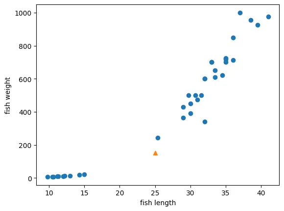

k-최근접 이웃의 다수결 원칙

→ 이웃된 5개의 샘플을 선택

distances, indexes = kn.kneighbors([[25, 150]])
print(indexes)

'''
[[21 33 19 30  1]]

이 샘플들로만 다시 시각화

# 시각화
import matplotlib.pyplot as plt

plt.scatter(train_input[:, 0], train_input[:, 1])
plt.scatter(25, 150, marker='^')
plt.scatter(train_input[indexes, 0], train_input[indexes, 1], marker='D')
plt.xlabel('fish length')
plt.ylabel('fish weight')
plt.show()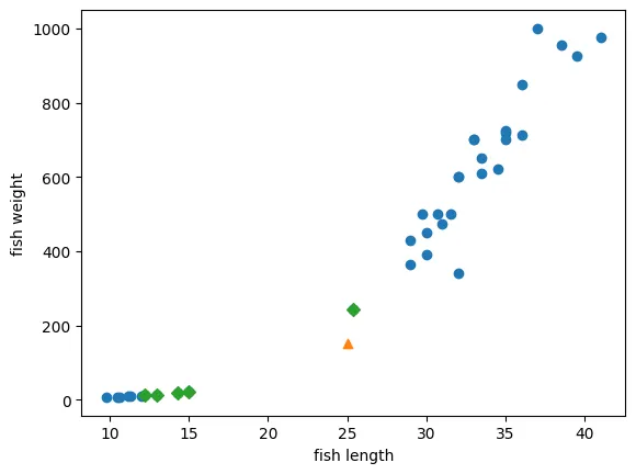

샘플 데이터 확인

print(train_input[indexes])

'''
[[[ 25.4 242. ]
  [ 15.   19.9]
  [ 14.3  19.7]
  [ 13.   12.2]
  [ 12.2  12.2]]]

하나 빼고 모두 빙어 데이터

샘플 데이터와 예측 데이터 간의 거리 계산

print(distances)

'''
[[ 92.00086956 130.48375378 130.73859415 138.32150953 138.39320793]]

하나만 특히 가까움

유클리디안으로 직선 거리 계산을 하므로 하나의 가중치에선 크고? 하나의 가중치에선 작으면? 별로 차이가 안나보인다?

가중치 업데이트가 필요?

여튼 정규화, 일반화를 안해주면 데이터에서 이상치가 더 잘나옴

5. 정규화

min-max, score

StatndardScaler : 평균, 표준편차 계산

# 5. 정규화
from sklearn.preprocessing import StandardScaler

sc = StandardScaler()

sc.fit(train_input)
scaled_input = sc.transform(train_input)

print(scaled_input)

fit() 으로 구한 평균, 표준편차로 transform 을 통해 데이터 정규화

정규화된 데이터로 재학습

kn.fit(scaled_input, train_target)

테스트용 데이터도 정규화 진행

new = sc.transform([[25, 150]])

print(kn.predict(new))

'''
[1.]

원하던 도미 데이터로 나옴

6. 알고리즘 검증

5개 이웃 샘플

distances, indexes = kn.kneighbors(new)

시각화

# 시각화
plt.scatter(scaled_input[:, 0], scaled_input[:, 1])
plt.scatter(new[0,0], new[0,1], marker='^')
plt.scatter(scaled_input[indexes, 0], scaled_input[indexes, 1], marker='D')
plt.xlabel('fish length')
plt.ylabel('fish weight')
plt.show()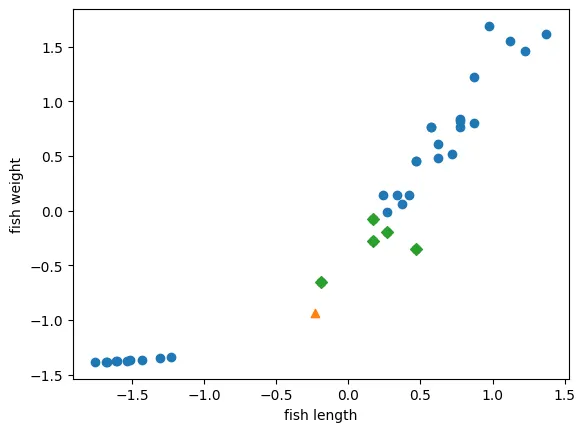

5개의 이웃 샘플이 이번엔 도미쪽으로 올바르게 잡힌 것을 확인 가능

모델 학습 전에 데이터 전처리(정규화 등) 필요!

K-최근접 이웃 회귀

데이터 준비

perch_length = np.array(
    [8.4, 13.7, 15.0, 16.2, 17.4, 18.0, 18.7, 19.0, 19.6, 20.0,
     21.0, 21.0, 21.0, 21.3, 22.0, 22.0, 22.0, 22.0, 22.0, 22.5,
     22.5, 22.7, 23.0, 23.5, 24.0, 24.0, 24.6, 25.0, 25.6, 26.5,
     27.3, 27.5, 27.5, 27.5, 28.0, 28.7, 30.0, 32.8, 34.5, 35.0,
     36.5, 36.0, 37.0, 37.0, 39.0, 39.0, 39.0, 40.0, 40.0, 40.0,
     40.0, 42.0, 43.0, 43.0, 43.5, 44.0]
     )
perch_weight = np.array(
    [5.9, 32.0, 40.0, 51.5, 70.0, 100.0, 78.0, 80.0, 85.0, 85.0,
     110.0, 115.0, 125.0, 130.0, 120.0, 120.0, 130.0, 135.0, 110.0,
     130.0, 150.0, 145.0, 150.0, 170.0, 225.0, 145.0, 188.0, 180.0,
     197.0, 218.0, 300.0, 260.0, 265.0, 250.0, 250.0, 300.0, 320.0,
     514.0, 556.0, 840.0, 685.0, 700.0, 700.0, 690.0, 900.0, 650.0,
     820.0, 850.0, 900.0, 1015.0, 820.0, 1100.0, 1000.0, 1100.0,
     1000.0, 1000.0]
     )

시각화

import matplotlib.pyplot as plt

plt.scatter(perch_length, perch_weight)
plt.xlabel('perch length')
plt.ylabel('perch weight')
plt.show()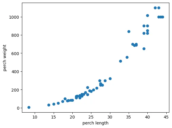

데이터 분할

# 데이터 분할
from sklearn.model_selection import train_test_split

train_input, test_input, train_target, test_target = train_test_split(perch_length, perch_weight, 
                                                                      random_state=42)

print(train_input.shape)
print(test_input.shape)

'''
(42,)
(14,)                                                                      

길이로 무게를 예측할 것이므로, 데이터셋 분할할 때도 length = input, weight = target 으로 넣어서 분할

현재 1차원 배열인 것을 확인 가능
→ 1차원 배열은 특성이 여러개 있는 것으로 판단하므로 2차원 배열로 변환이 필요함

데이터 형태를 확인 후 2차원 배열로 변환

train_input = train_input.reshape(-1, 1)
test_input = test_input.reshape(-1, 1)

print(train_input.shape)
print(test_input.shape)

'''
(42, 1)
(14, 1)

이제 특성 1개에 샘플이 여러개 있는 형태로 변환됨

📌

k-최근접 이웃 회귀, 평가

1. 결정계수

   $R^2 = 1 - \frac{\sum_{i=1}^{n} (y_i - \hat{y}_i)^2}{\sum_{i=1}^{n} (y_i - \bar{y})^2}$

   𝑦̄: 실제 값들의 평균

   $R^2=1$
   → 완벽한 예측

   $R^2=0$
   → 분산 이해가 낮음

   $R^2=7..$
   → 똥!

   📌

   $R^2<0$ (결정계수가 음수일 경우) 체크리스트

   • train/test input 점검, 라벨이 밀리지 않았는지
   • 시각화 → 상관관계를 확인
   • 스케일링 확인
   • 학습/평가 파이프라인 확인
   • 모델 구조 복잡성 확인

결정계수가 1에 가까울 수록 예측 정확도가 높다

2. mae 확인

   : Mean Absolute Error(평균 절댓값 오차)

   : 실제 값과 모델이 예측한 값 사이의 절대적인 차이를 모두 더한 후, 그 평균을 낸 값

   $\text{MAE} = \frac{1}{n} \sum_{i=1}^{n} |y_i - \hat{y}_i|$

   예측 오차의 평균 크기를 나타내며, 값이 작을수록 모델의 예측 성능이 좋다는 것을 의미함

k-최근접 이웃 평가 지표

k-최근접 이웃 회귀 학습기 생성

from sklearn.neighbors import KNeighborsRegressor

knr = KNeighborsRegressor()
knr.fit(train_input, train_target)

학습기 평가 지표 확인 - 1. 정확도(결정계수)

print(knr.score(train_input, train_target))
print(knr.score(test_input, test_target))

'''
0.9698823289099254
0.992809406101064

과소적합이 일어나긴 했으나 큰 문제가 되는 수치는 아님

학습기 평가 지표 확인 - 2. mae

prediction value 와 target value 사이의 평균 절댓값 오차

from sklearn.metrics import mean_absolute_error

test_prediction = knr.predict(test_input)
mae = mean_absolute_error(test_target, test_prediction)

print(mae)

'''
19.157142857142862

예측 값(예측한 perch 의 무게)와 평균적으로 19그램 차이 남

관점에 따라 다르지만
데이터 분포를 보면 19그램 정도는 무난한 값이라고 판단할 수도 있음

과대적합 vs 과소적합

과대적합

print(knr.score(train_input, train_target))
print(knr.score(test_input, test_target))

# 이웃의 개수를 3개로 줄이기
knr.n_neighbors = 3

# 재훈련
knr.fit(train_input, train_target)

# 정확도(결정계수) 다시 확인
print(knr.score(train_input, train_target))
print(knr.score(test_input, test_target))

'''
0.9698823289099254
0.992809406101064
0.9804899950518966
0.9746459963987609

학습셋 정확도 96, 테스트셋 정확도 99 로 테스트셋 정확도가 더 높을 땐 과소적합

학습셋 정확도 98, 테스트셋 정확도 97 로 학습셋 정확도가 더 높을 땐 과대적합

과대적합 그래프

# 과대적합 그래프
knr = KNeighborsRegressor()

# 1 ~ 44, length 의 모든 범위 커버 가능
x = np.arange(1, 45).reshape(-1, 1)

# 이웃의 개수 1, 5, 10 인 경우 비교
for n in [1, 5, 10]:
  knr.n_neighbors = n
  knr.fit(train_input, train_target)
  
  prediction = knr.predict(x)

  plt.scatter(train_input, train_target)
  plt.plot(x, prediction)
  plt.xlabel("length")
  plt.ylabel("weight")
  plt.show()

이웃의 개수 1, 5, 10 인 경우 비교

이웃의 개수 = 1

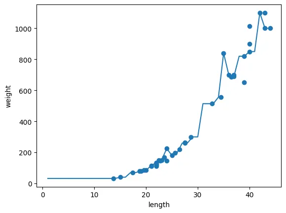
각 샘플을 다 따라가려고 지그재그
→ 과대적합

이웃의 개수 = 5

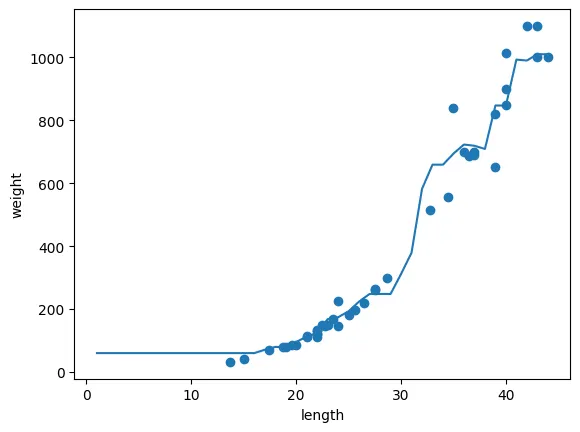
좀 더 완만해짐

이웃의 개수 = 10

📌

k-최근접 이웃 과대적합 해결책

이웃의 개수 늘리기

k-최근접 이웃 한계

# 50cm인 농어의 무게 예측 및 이웃(3)을 포함한 시각화
# 이웃 3인 학습기 생성
from sklearn.neighbors import KNeighborsRegressor
import matplotlib.pyplot as plt

knr = KNeighborsRegressor(n_neighbors = 3)

#  학습
knr.fit(train_input, train_target)

print(knr.predict([[50]]))

# 거리, 이웃 구하기
distances, indexes = knr.kneighbors(x)

# 시각화
plt.scatter(train_input, train_target)
plt.scatter(train_input[indexes, :], train_target[indexes], marker='D')
plt.scatter(50, 1033, marker='^')
plt.xlabel("length")
plt.ylabel("weight")
plt.show()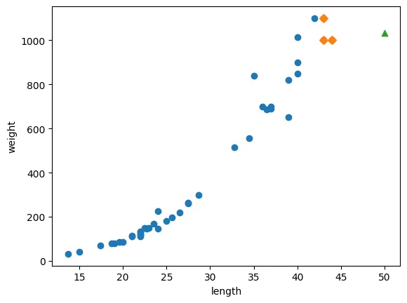

평균값과 예측값 확인

print(np.mean(train_target[indexes]))
print(knr.predict([[50]]))

'''
1033.3333333333333
[1033.33333333]

길이가 100 인 농어의 무게 예측

print(knr.predict([[100]]))

'''
[1033.33333333]

# 100cm인 농어의 무게 예측 및 이웃(3)을 포함한 시각화
# 이웃 3인 학습기 생성

# 거리, 이웃 구하기
distances, indexes = knr.kneighbors([[100]])

# 시각화
plt.scatter(train_input, train_target)
plt.scatter(train_input[indexes, :], train_target[indexes], marker = 'D')
plt.scatter(100, 1033, marker = '^')
plt.xlabel('length')
plt.ylabel('weight')
plt.show()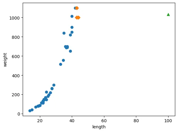

아무리 길이가 떨어진 이상치여도 가장 가까운 이웃들의 타겟 값을 기준으로 평균을 계산함

선형회귀

# 선형회귀
from sklearn.linear_model import LinearRegression

lr = LinearRegression()

lr.fit(train_input, train_target)

선형회귀로 구한 예측값 확인

print(lr.predict([[50]]))

'''
[1241.83860323]

기울기, 절편 구하기

print(lr.coef_, lr.intercept_)

'''
[39.01714496] -709.0186449535477

시각화

plt.scatter(train_input, train_target)
plt.plot([15, 50], [15 * lr.coef_ + lr.intercept_, 50 * lr.coef_ + lr.intercept_])
plt.scatter(50, 1241.8, marker='^')
plt.xlabel('length')
plt.ylabel('weight')
plt.show()

점 두 개 잡아서 그래프 그려보기

평가

print(lr.score(train_input, train_target))
print(lr.score(test_input, test_target))

다항 회귀

다항 ≠ 다차항

$x^2$ 이 새로운 매개변수 z 와 같음

poly: 다항

train_poly = np.column_stack((train_input ** 2, train_input))
test_poly = np.column_stack((test_input ** 2, test_input))

print(train_input.shape)
print(train_poly.shape)

'''
(42, 1)
(42, 2)

$x^2$, x 값을 넣어서 선형 회귀 학습

lr = LinearRegression()

lr.fit(train_poly, train_target)

print(lr.predict([[50**2, 50]]))

'''
[1573.98423528]

기울기, 절편 구하기

# 기울기 2개, 절편 구하기
print(lr.coef_, lr.intercept_)

'''
[  1.01433211 -21.55792498] 116.0502107827827

시각화

point = np.arange(15, 51)

plt.scatter(train_input, train_target)
plt.plot(point, 1.01 * (point ** 2) - 21.5 * point + 116)
plt.scatter(50, 1574, marker='^')
plt.xlabel('length')
plt.ylabel('weight')
plt.show()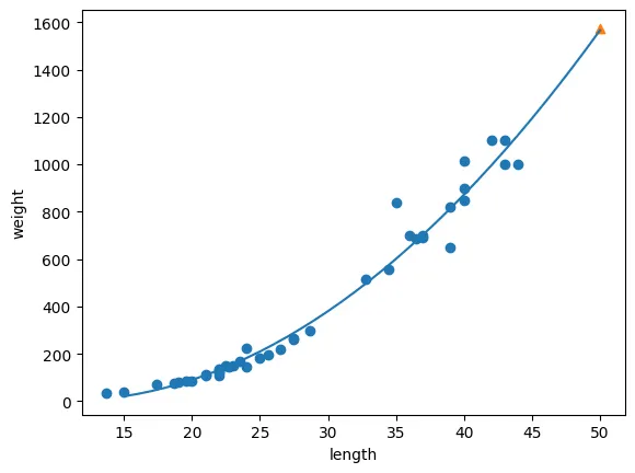

점수

# 점수
print(lr.score(train_poly, train_target))
print(lr.score(test_poly, test_target))

'''
0.9706807451768623
0.9775935108325122

📌

다차항 = 특성 공학

위와 같이 3개의 특성을 가진 데이터에서 모델이 더 잘 학습하도록 데이터를 새로운 특징(feature)으로 변환하거나 생성

⇒ x, y, z, xy, xz, yx, x^2, y^2, x^2 9개의 특성

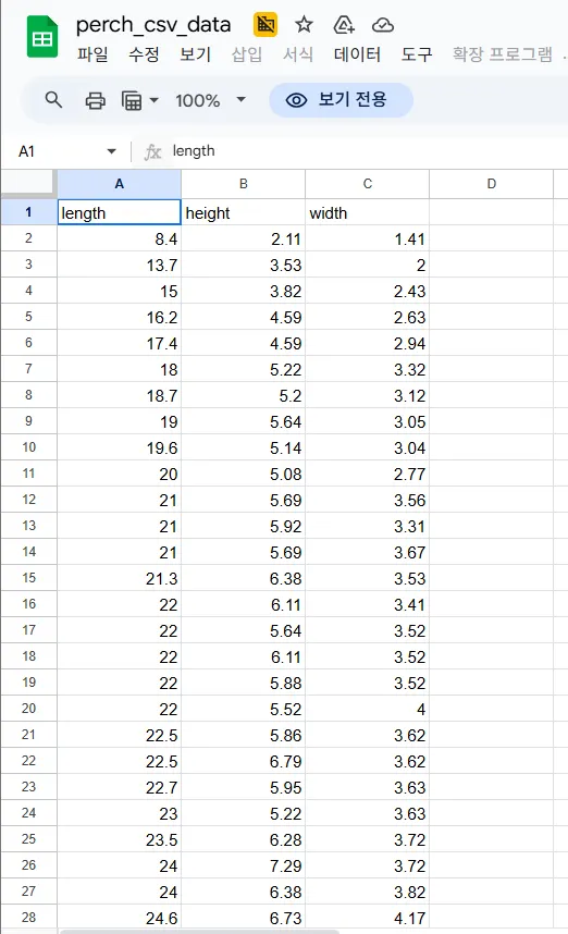
# 다차항 = 특성 공학
import pandas as pd

perch_full = pd.read_excel('perch_csv_data.xlsx')
print(perch_full.head())

'''
   length  height  width
0     8.4    2.11   1.41
1    13.7    3.53   2.00
2    15.0    3.82   2.43
3    16.2    4.59   2.63
4    17.4    4.59   2.94

무게 데이터

import numpy as np

perch_weight = np.array(
    [5.9, 32.0, 40.0, 51.5, 70.0, 100.0, 78.0, 80.0, 85.0, 85.0,
     110.0, 115.0, 125.0, 130.0, 120.0, 120.0, 130.0, 135.0, 110.0,
     130.0, 150.0, 145.0, 150.0, 170.0, 225.0, 145.0, 188.0, 180.0,
     197.0, 218.0, 300.0, 260.0, 265.0, 250.0, 250.0, 300.0, 320.0,
     514.0, 556.0, 840.0, 685.0, 700.0, 700.0, 690.0, 900.0, 650.0,
     820.0, 850.0, 900.0, 1015.0, 820.0, 1100.0, 1000.0, 1100.0,
     1000.0, 1000.0]
     )

데이터 분할

# 훈련용, 테스트용 데이터 분할
train_input, test_input, train_target, test_target = train_test_split(perch_full, perch_weight,
                                                                      random_state = 42)

# 훈련용, 테스트용 데이터 분할
train_input, test_input, train_target, test_target = train_test_split(perch_full, perch_weight,
                                                                      random_state = 42)

특성 공학은 가중치를 다양하게 부여해주는 것을 의미

기본 차수는 2

# 특성 공학은 가중치를 다양하게 부여해주는 것을 의미
# 기본 차수는 2
from sklearn.preprocessing import PolynomialFeatures

poly = PolynomialFeatures()

poly.fit([[2, 3]])
print(poly.transform([[2, 3]]))

'''
[[1. 2. 3. 4. 6. 9.]]

1 = 상수항

2 = 2

3 = 3

4 = 2 ** 2

6 = 2 * 3

9 = 3 ** 2

상수항 1 생략

poly = PolynomialFeatures(include_bias=False)

poly.fit([[2,3]])
print(poly.transform([[2,3]]))

'''
[[2. 3. 4. 6. 9.]]

특성 공학으로 데이터셋의 원래 특성을 이용해 새로운 특성 생성

poly = PolynomialFeatures(include_bias=False)

poly.fit(train_input)
train_poly = poly.transform(train_input)

print(train_poly.shape)

'''
(42, 9)

x, y, z, xy, xz, yx, x^2, y^2, x^2
⇒ 총 9개

특성 공학의 특성 조합 확인

print(poly.get_feature_names_out())

'''
['length' 'height' 'width' 'length^2' 'length height' 'length width'
 'height^2' 'height width' 'width^2']

테스트 셋도 특성 생성

test_poly = poly.transform(test_input)

선형 회귀

lr = LinearRegression()

lr.fit(train_poly, train_target)

점수 확인

print(lr.score(train_poly, train_target))
print(lr.score(test_poly, test_target))

'''
0.9903183436982125
0.9714559911594111

과대적합이 일어나긴 했으나 준수한 결과

특성 공학을 5차까지 증가

특성 공학의 차수를 증가 → 데이터의 복잡성 증가

# 특성 공학을 5차까지 증가
poly = PolynomialFeatures(degree=5, include_bias=False)

poly.fit(train_input)
train_poly = poly.transform(train_input)
test_poly = poly.transform(test_input)

print(poly.get_feature_names_out())
print(train_poly.shape)

'''
['length' 'height' 'width' 'length^2' 'length height' 'length width'
 'height^2' 'height width' 'width^2' 'length^3' 'length^2 height'
 'length^2 width' 'length height^2' 'length height width' 'length width^2'
 'height^3' 'height^2 width' 'height width^2' 'width^3' 'length^4'
 'length^3 height' 'length^3 width' 'length^2 height^2'
 'length^2 height width' 'length^2 width^2' 'length height^3'
 'length height^2 width' 'length height width^2' 'length width^3'
 'height^4' 'height^3 width' 'height^2 width^2' 'height width^3' 'width^4'
 'length^5' 'length^4 height' 'length^4 width' 'length^3 height^2'
 'length^3 height width' 'length^3 width^2' 'length^2 height^3'
 'length^2 height^2 width' 'length^2 height width^2' 'length^2 width^3'
 'length height^4' 'length height^3 width' 'length height^2 width^2'
 'length height width^3' 'length width^4' 'height^5' 'height^4 width'
 'height^3 width^2' 'height^2 width^3' 'height width^4' 'width^5']
(42, 55)

print(lr.score(train_poly, train_target))
print(lr.score(test_poly, test_target))

'''
0.9999999999996433
-144.40579436844948

데이터의 복잡성이 증가하면 예측도 어려움