머신러닝-2단계(성능평가)

1. 성능평가

• 회귀 모델 성능 평가
  • 예측 값과 실제 값의 차이(오차) : SSE가 적어야 한다.
  • 예측 값과 실제 값의 평균 : SSR이 커야 한다.
  • 예측 값이 실제 값에 가까울수록 좋은 모델이다.

---

• 분류 모델 성능 평가
  • accuray, recall, precision이 커야 한다.
  • 예측 값이 실제 값과 같을 수록 좋은 모델이다.

2. 회귀 모델 성능 평가

1) MAE(Mean Absolute Error)
$\large MAE=\frac{1}{n}\sum_{i=1}^{n}|y_{i}-\hat{y}_{i}|$
<모듈>
from sklearn.metrics import mean_absolute_error

2) MAPE(Mean Absolute Percentage Error)
$\large MAPE=\frac{1}{n}\sum_{i=1}^{n}\left |\frac{y_{i}-\hat{y}_{i}}{y_{i}}\right |$
<모듈>
from sklearn.metrics import mean_absolute_percentage_error

3) MSE(Mean Squared Error)
$\large MSE=\frac{1}{n}\sum_{i=1}^{n}(y_{i}-\hat{y}_{i})^2$
<모듈>
from sklearn.metrics import mean_squared_error

4) RMSE(Root Mean Squared Error)
<모듈>
from sklearn.metrics import mean_squared_error
<성능 평가>
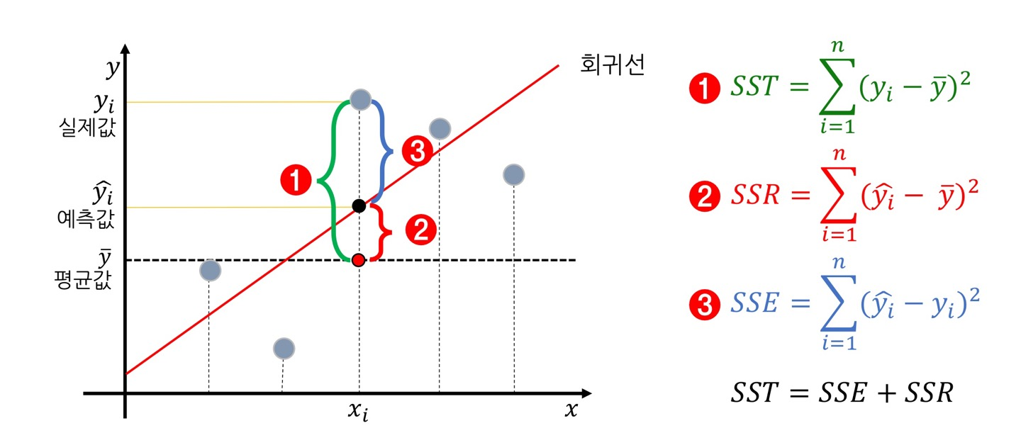
print('MSE :', mean_squared_error(y_test, y_pred)**0.5)

5) SST = SSE + SSR

• SSE : 회귀식이 여전히 잡아내지 못한 오차
• SSR : 회귀식이 잡아낸 오차
• SSE는 작을수록 좋고 SSR은 클수록 좋다. 즉, SST == SSR을 목표한다.
  cf) SSR 대신에 SSE가 쓰이는 경우도 있는데 이때의 SSE는 잔차에 관한 것이다.
  

6) R2-Score
$\large R^2=1-\frac{SSE}{SST}=1-\frac{\sum_{i=1}^{n}(y_{i}-\hat{y}_{i})^2}{\sum_{i=1}^{n}(y_{i}-\bar{y}_{i})^2}$
<모듈>
from sklearn.metrics import r2_score
<성능 평가>
방법 1) print('R2 :', r2_score(y_test, y_pred))
방법 2) print(model.score(x_test, y_test))

cf) model.score()는 회귀 문제에서 R2와 같다.

<해석>
R2 = 0.85 이면, 우리의 모델이 평균보다 85% 더 설명력이 있다.

---

---

3. 분류 모델 성능 평가

1) Confusion Matrix <crosstab과 같음>

# 모듈 
from sklearn.metrics import confusion_matrix
# 성능 평가
print(confusion_matrix(y_test, y_pred))
<출력>
			예측값 0 예측값 1
실제값 0		[[76 	 8]
실제값 1 	[16 	50]]

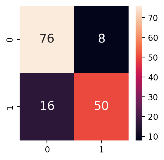
2) 혼동행렬 시각화

sns.heatmap(confusion_matrix(y_test, y_pred),
           annot=True, 
           annot_kws={'size' : 15})

3) Accuracy
$\large Accuracy = \frac{TP+TN}{TP+TN+FP+FN}$

# 모듈
from sklearn.metrics import accuracy_score
# 성능 평가
방법 1) print(accuracy_score(y_test, y_pred))
방법 2) model.score(x_train, y_train)
<출력>
[0.82608696 0.86206897]

4) Precision
$\large Precision = \frac{TP}{TP+FP}$

• 예측값을 기준으로 true인 것

# 모듈
from sklearn.metrics import precision_score
# 성능 평가
precision_score(y_test, y_pred, average = None)
<출력>
[0.82608696 0.86206897]

5) Recall
$\large Recall = \frac{TP}{TP+FN}$

• 실제값을 기준으로 true인 것

# 모듈
from sklearn.metrics import recall_score
# 성능 평가
recall_score(y_test, y_pred, average = None)
<출력>
[0.9047619  0.75757576]

cf) specificity(특이도)
$\large Recall = \frac{TN}{TN+FP}$

• 실제값의 Negative 중 true인 것

6) F1-Score
$\large F1 = \frac{2\times Precision\times Recall}{Precision+Recall}$

# 모듈
from sklearn.metrics import f1_score
# 성능 평가
print(f1_score(y_test, y_pred, average = None))
<출력>
[0.86363636 0.80645161]

7) Classification Report

# 모듈
from sklearn.metrics import classification_report
# 성능 평가
classification_report(y_test, y_pred)
<출력>
             precision    recall  f1-score   support

           0       0.83      0.90      0.86        84
           1       0.86      0.76      0.81        66

    accuracy                           0.84       150
   macro avg       0.84      0.83      0.84       150
weighted avg       0.84      0.84      0.84       150