2. Bayesian Decision Theory

1. Pattern Discovery in Data

데이터에서 규칙성을 찾는 것은 고전 역학부터 양자 역학에 이르기까지 과학 발전의 근간이 되어온 중요한 문제이다.

1.1 Pattern Recognition

• automatically discover regualarities in data
• and use these regualarities to make decision
• e.g., classifying the data into different categories
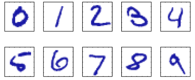
  • handwritten digit recognition

1.2 Machine Learning

• a large set of input vectors $x_1, ..., x_N$, or a training set is used
  • to tune the parameters of an adaptive model
• the category of an input vector is expressed using a target vector $t$
• the result of algorithm: $y(x)$ where the output $y$ is encoded as target vectors

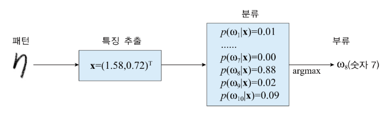
입력 $x$는 숫자 이미지의 각 픽셀 값들이고, 타겟 벡터 $t$는 모델이 도달해야 하는 목표, 해당 이미지의 실제 정답을 의미한다.

1.3 Why Probability is Important in Data Mining

Goal

• discover meaningful patterns from large datasets

Challenge

• real-word data is urcentain and noisy due to measurement errors or incomplete information

Solution

• Probability theory provides a mathematical framework to model and reason about uncertainty

Applications

• key tasks rely on probabilistic reasoning
  • clssification, clustering
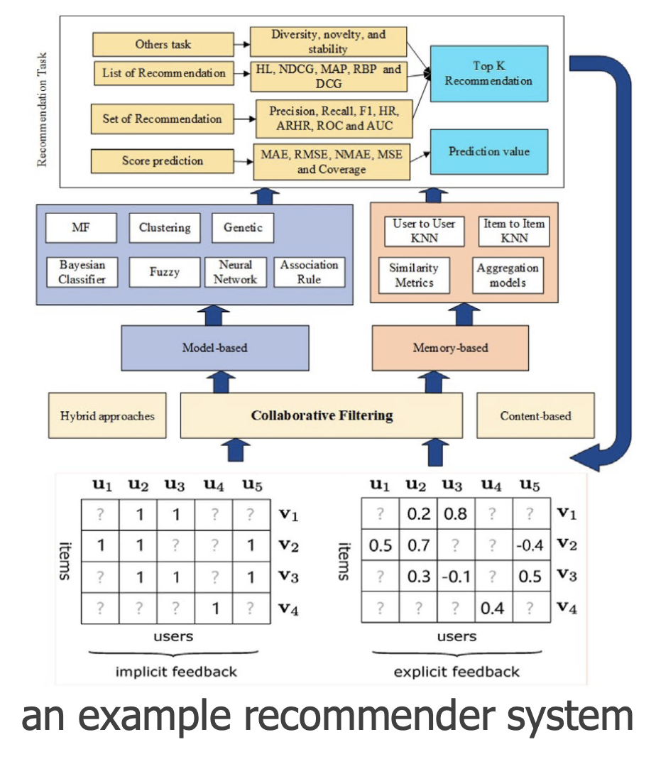
  • recommendation systems
  • anomaly detection
  • predictive modeling

Benefit

• allows us to quantify uncertainty and make informed decisions
• e.g.,
  • spam detection
  • purchase likelihood

확률로 불확실성을 정량화하고 위험을 종합적으로 따져 논리적인 결론을 도출한다.

---

2. Basic Concept of Probability

2.1 Fundamentals

Experiment

• a process that produces outcomes that cannot be predicted with certainty
• e.g., tossing a coin, rolling a die

Sample Space $S$

• the set of all possible outcomes of an experiment
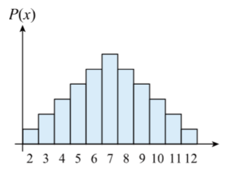
• e.g., die roll $S = {1, 2, 3, 4, 5, 6}$

Event

• a subset of the sample space representing outcomes of interest
• e.g., even number $A = {2, 4, 6}$

2.2 Conditional Probability

• the probability of event $A$ occuring given that event $B$ has already occurred
• the formula is $P(A|B) = P(A \cap B)/P(B)$ provided that $P(B)>0$

2.3 Random Variables

• a function that assigns a numerical value to the outcome of a random experiment

1. Discrete Random Variable

• takes a finite or countably infinite set of values
• described by a probability mass function(PMF)

2. Continous Random Variable

• takes any value within an interval
• described by a probability density function(PDF)

Importance

• they translate real-word uncertainty into mathematics forms to compute expectation and variance for decision-making

2.4 Independence

• two events $A$ and $B$ are independent
• the occurrence of one does not affect the probability of the other
  • $P(A|B) = P(A)$
  • equivalently $P(A \cap B) = P(A)P(B)$

In Data Mining

• Naive Bayes assumes features are conditionally indepedent given the label to simplify calculations
• e.g., email classification features

사실 현실에서는 "free"와 "win" 같은 단어가 스팸 메일에 함께 자주 등장하므로 이 가정은 비현실적이다. 하지만 계산을 단순화해도 뛰어난 성능을 보이기 때문에 널리 사용한다.

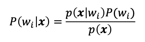
2.5 Bayes' Theorem

Prior Probability $P(X)$

• initial belief about an event before observing any evidence

초기의 믿음, 가진 정보를 의미한다.

Likelihood $P(Y|X)$

• the probability of observing evidence $Y$ given that hypothesis $X$ is true
• how well the hypothesis explains the observed data

Posterior Probability $P(X|Y)$

• the probability of an event after observing evidence
• it updates the prior probability using new information

새로운 정보를 이용해서 사전 확률을 업데이트하는 과정이다.

Bayes' Theorem

$\displaystyle P(X|Y) = \frac{P(Y|X)P(X)}{P(Y)}$

• $P(Y)$: marginal probability(nomalization constant) calculated as $\sum P(Y|X_i)P(X_i)$

한계 확률 또는 정규화 상수라고 불리며 관찰된 증거가 나타날 전체 확률을 의미한다. 위 식에서 분자만 계산하면 합이 1이 되지 않을 수 있기에 $P(Y)$로 나누어 결과값들을 0과 1 사이로 맞춘다.
$\rightarrow$ 정규화 상수

E.g.,

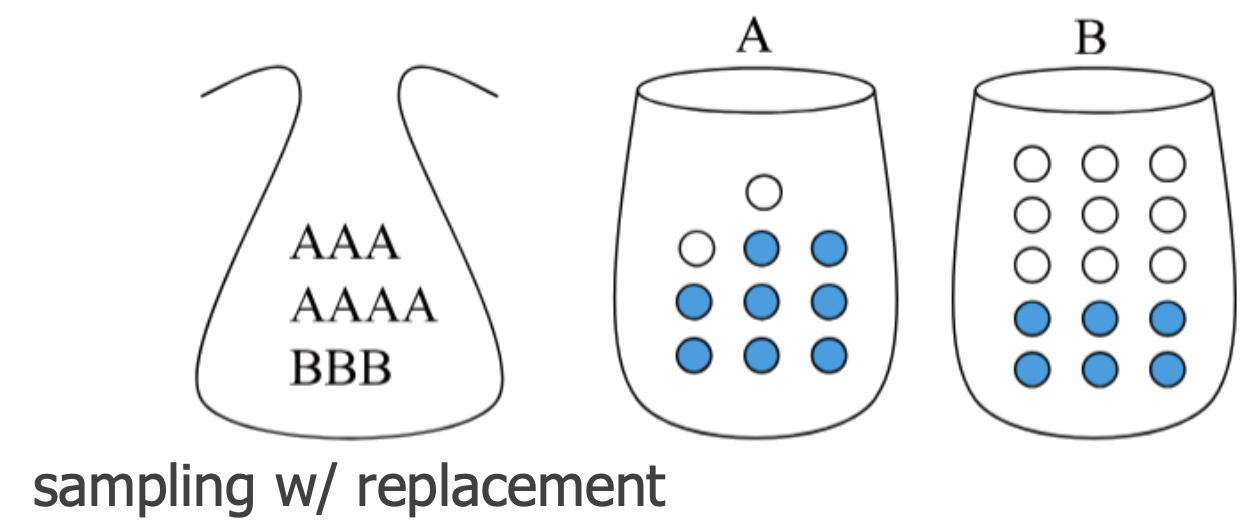
• joint Probability: P(A,white)
• marginal Probability: P(white)
• posterior Probability: P(A∣white)
  • updating the probability of choosing Bag A after seeing a white ball

---

3. Bayesian Decision Theory

Definition

• a fundamental statistical approach to learning from data
  • quantify the trade-offs between different decisions using probabilities and associated costs

확률과 각 결정에 따르는 비용을 이용해 서로 다른 의사결정 간의 trade-off를 정량화하는 데 기반한다.

Assumptions

• problems are posed in probabilistic terms, and all relevant probability values are known

E.g.,

• sorting fish based on features
  • sea bass vs. salmon

전형적인 베이지안 결정 이론 예제로 관찰된 특징(무게, 길이, 색상)에 대한 조건부 확률을 이용해 어느 클래스에 속할지 결정한다.

관찰된 데이터(특징 $x$)가 주어졌을 때, 각 클래스($w_i$)의 likelihood를 측정한다.

---

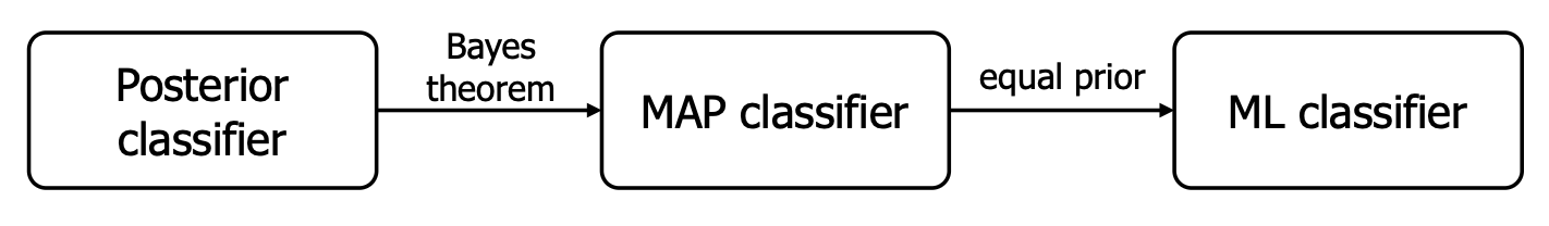
4. Bayesian Classifier

4.1 Posterior Classifier

• = Bayes Classifier
• assign observation $x$ to the class $w_i$ with the highest posterior probability $P(w_i | x)$

$p(w_i|x)$: posterior probability
$p(x|w_i)$:: likelihood
$p(w_i)$: prior probability
$p(x)$: evidence

Binary Classification

• $P(w_1|x) > P(w_2|x)$, then classify $x$ belongs to $w_1$
• $P(w_1|x) < P(w_2|x)$, then classify $x$ belongs to $w_2$

4.2 MAP Classifier

• computing the posterior probability directly is difficult
  • since the evidence $p(x)$ is constant for all classes, it can be ignored during comparison
• choose the class with the largest $p(x|w_i)P(w_i)$(likelihood $\times$ prior)

Binary Classification

• $p(x|w_1)P(w_1) > p(x|w_2)P(w_2)$, then classify $x$ belongs to $w_1$
• $p(x|w_1)P(w_1) < p(x|w_2)P(w_2)$, then classify $x$ belongs to $w_2$

Bayes classifier에서 어차피 비교만 할 거면 p(x)를 계산할 필요가 없어, p(x)를 생략하고 likelihood x prior만 비교한다.

4.3 ML Classifier

• if we have the same prior, we can omit $P(w_1)$ and $P(w_2)\rightarrow$ Maximum Likelihood Classifier
• choose the class with the larget likelihood: $argmax_i p(x|w_i)$

$p$: PDF(연속형 확률 변수)
$P$: PMF(이산형 확률 변수)
$P(w_i|x)$: 연속적인 $x$를 관측했을 때, 이 물고기가 어떤 이산적 클래스$w_i$에 속할 확률

Classifier	Decision Rule	Meaning
Posterior Classifier	$argmax_i p(w_i \mid x)$	최고 사후 확률 클래스 선택 [1, 3]
MAP Classifier	$argmax_i p(x \mid w_i)p(w_i)$	우도(Likelihood) × 사전 확률(Prior) [1-3]
ML Classifier	$argmax_i p(x \mid w_i)$	우도(Likelihood)만 고려 [2, 3]

---

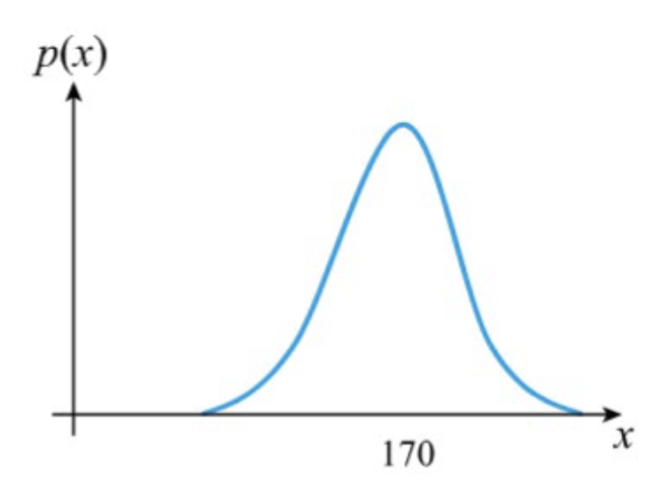
4.4 Error Probability

• even with the most optimal classifier, errors are unavoidable whenever class districutions overlap

Definition

• the probability that a classifier assigns a sample to the wrong decision region

Decision Regions $R_1, R_2$

• these denote the areas in the feature space assigned to specific classes
• e.g., if a sample fails in $R_1$, it is classified as $w_1$

오류 확률은 샘플이 실제 속한 클래스가 아닌 잘못된 결정 영역에 할당된 확률이다.

General Formula

• assuming two districutions have the same prior, the error $E$ calculated as

$E = \frac{1}{2} \int_{-\infty}^{t} p(x|w_2)dx + \frac{1}{2} \int_{t}^{\infty} p(x|w_1)dx$

• the integrals measure the misclassified probability mass, which is represented by the shared area in the distribution graph

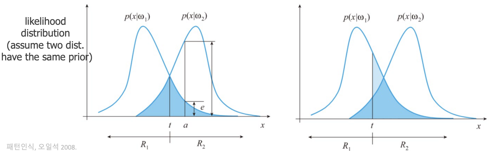
• the level of overlap between the likelihood distributions $p(x|w_1)$ and $p(x|w_2)$ is critical
• the more they overlap, the higher the error rate will be

---

5. Minimum Risk Bayesian Classifier

5.1 Beyond Error Rate: Expected Risk

The problem with Error Rate

• minimizing the error rate implicitly assumes that every mistake costs the same

The Reality

• in practice, different errors have different consequences
  • e.g., false alarms vs. missed detections

The Goal

• incorporate these different "loss" values into the decision-making process to minimize the Expected Risk rather than just the number of errors

5.2 Loss Matrix $C$

Definition

• a matrix that quantifies the penalty for every possible decision

Notation $c_{ij}$

• the loss incurred when the true class is $w_i$, but the classifier decides it is $w_j$
  • $c_{ii}$: correct decision (0 or very low cost)
  • $c_{ij}(i \ne j)$: incorrect decision (penalty > 0)

5.3 Conditional Risk for a Sample

• when we observe a sample $x$, we must choose between deciding $w_1$ or $w_2$
• $q_1$: the total risk we take by calling $x$ is a $w_1$
  • it considers both the chance that $x$ is actually $w_1$ (correct) and the chance it is $w_2$ (wrong)
  • $q_1 = R(w_1|x) = c_{11}p(x|w_1)P(w_1) + c_{21}p(x|w_2)P(w_2)$
• $q_2$: the risk of calling $x$ is a $w_2$
  • $q_2 = R(w_2|x) = c_{12}p(x|w_1)P(w_1) + c_{22}p(x|w_2)P(w_2)$

특정 결정을 했을 때 기대되는 손실을 conditional risk라고 부른다.

Decision Rule

• we decide $w_1$ if its risk is lower than $w_2$ $(q_1 < q_2$)

두 클래스 중 하나를 결정해야 할 때, 조건부 위험이 더 작은 쪽을 선택한다.

5.4 Likelihood Ratio

• by rearranging the inequality $q_2 > q_1$, we get the final decision rule based on the Likelihood Ratio

Likelihood Ratio

$\displaystyle \frac{p(x|w_1)}{p(x|w_2)} > \frac{(c_{21}-c_{22})P(w_2)}{(c_{12}-c_{11})P(w_1)}$

Thereshold

• the right-hand side is a constant value (independent of $x$)
• the classifier simply compares the ratio of the two likelihood against this threshold

우변은 미리 설정한 손실 비용과 사전 확률, 즉 상수이다. $x$에 대한 두 클래스의 우도비를 구한 뒤, 이미 계산해 둔 고정된 임계값보다 큰지 작은지만 확인하여 클래스를 결정한다.

5.5 Boundary Shifting

MAP as a Special Case

• if all misclassification costs are equal$(c_{12} = c_{21})$ and $c_{ii}=0$, this rule simplifies back to the MAP classifier

Shifting

• if the cost of misclassifying $w_1$ increases ($c_{12}$ gets larger), the thereshold becomes smaller
• this shifts the decision boundary to make it "easier" to classify something as $w_1$ to avoid the high cost of missing it

틀렸을 때 더 위험한 클래스가 있다면 thereshold를 낮춰서 더 적극적으로 찾아내도록 분류기를 조정한다.

---

6. Naive Bayes Spam Filter

classify emails as spam or non-spam using Bayes's theorem!

Naive Assumption

• features are assumed to occur independently given the class label to simplify calculation

단어들이 서로 독립이라고 가정하기 때문에 naive하다.

Parameter

• prior $P(spam)$: the proportion of spam emails in the total training set
  • $n(s)/n$
• likelihood $P(x_i|spam)$: the probability that word $w_i$ apeears in a spam email
  • $n(i, s)/n(s)$

Classification Rule

• calculate the posterior probability: $P(spam|x) \propto P(spam)$
• the email is classified as spam if this value is higher than the probability for non-spam class

Practicality

• although the independence assumption is often unrealistic, the method performs well in practice