4. Decision Tree (1)

1. Classification

1.1 Definition

• a data analysis task learns a model
  • classifier
• predicts categorical (discreate) class labels

E.g.,

• loan approaval
• medical diagnosis
• spam detection
• autonomous driving

Training

Evaluation & Prediction

사전에 정의된 클래스를 예측하는 모델(classifier)을 학습하는 것으로 입력 특징 $x \rightarrow$ 분류기 $\rightarrow \hat{y}$ 의 흐름으로 동작한다.

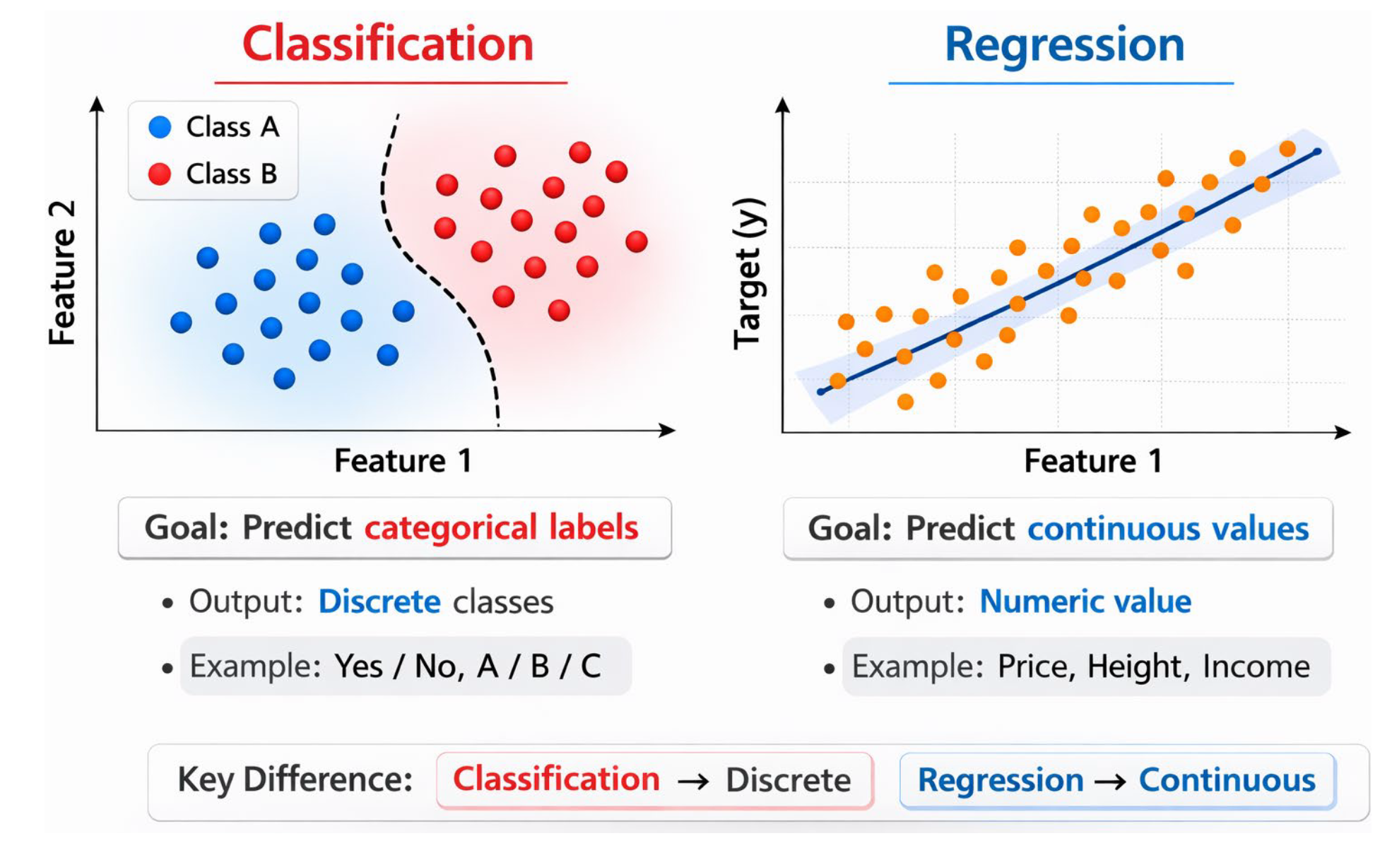
1.2 Classification vs. Prediction

Classification

• output: categorical labels
  • e.g., yes/no, pos/neg, class A, B, C

Numerical Prediction

• output: continous values
  • e.g., house price, income, sales amounts

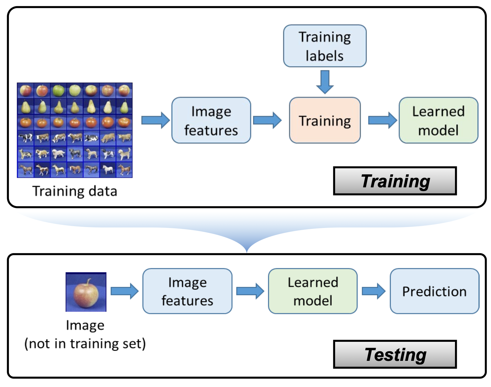
1.3 Supervised Learning

Setup

• input: feature vector $x$
• output: label $y$

Learning objective

• learning mapping from $x$ to $y$
• $f: x \rightarrow y$

Training data

• labeled dataset
• $D = {(x_1, y_1), ..., (x_n, y_n)}$

the model is learned from labeled data and then applied to unseen inputs

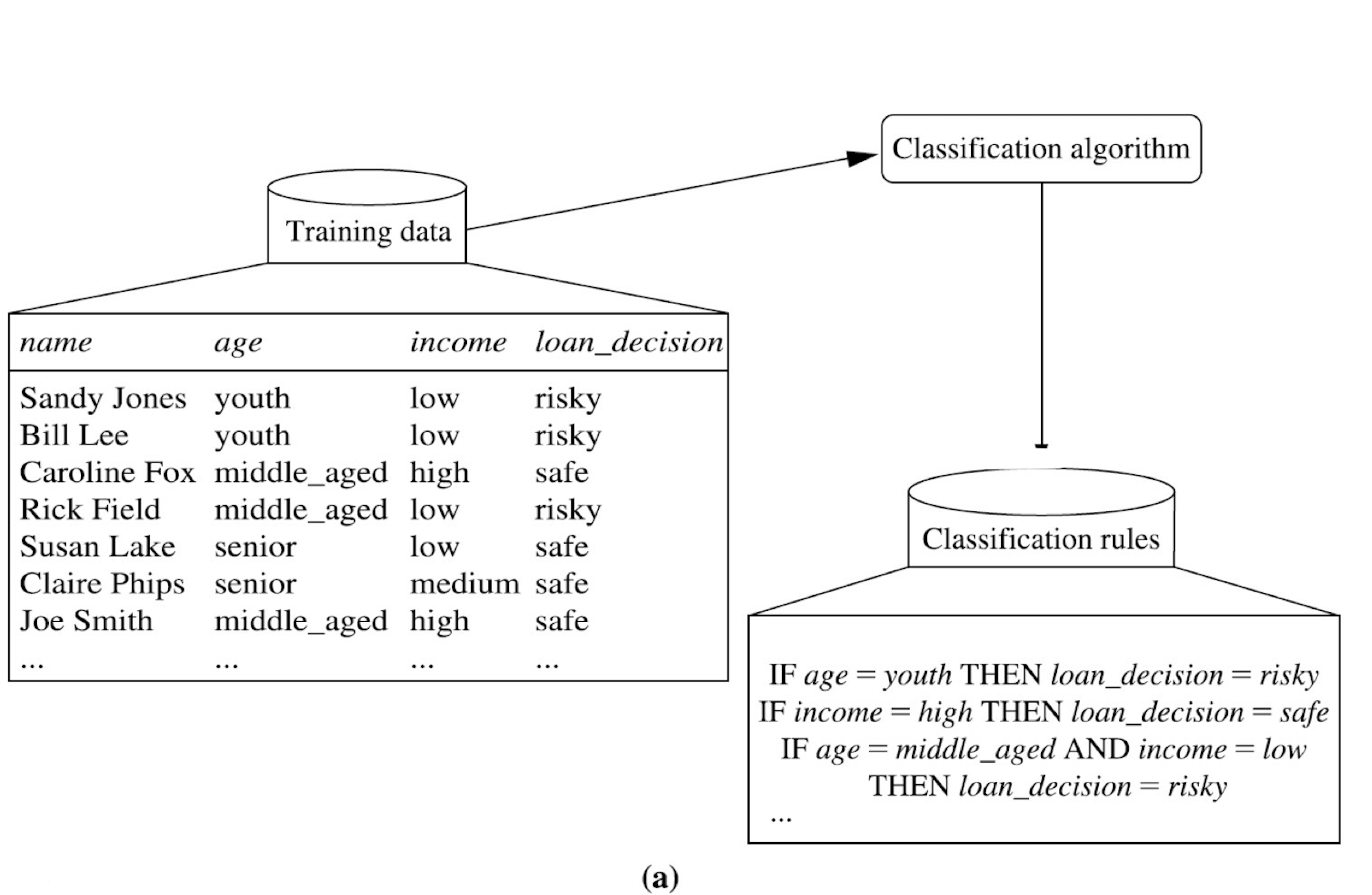
1.4 Process of Classification

1. Model Construction

• learn classifier from training data

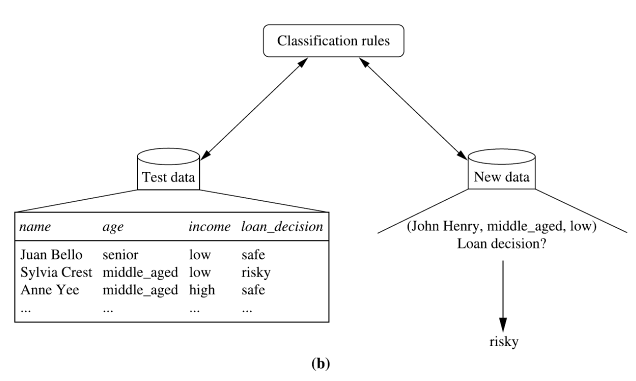
2. Model Evaluation

• test accuracy on unseen data
• if acceptable $\rightarrow$ deploy model

3. Prediction

• apply model to new data

Applications

• fraud detection
• medical diagnosis
• intrusion detection
• sentiment analysis
• recommendation systems

---

2. Decision Tree

2.1 Definition

• a supervised learning method for classification and regression
• predicts output $y$ from inputs $x \in \R^d$
• uses a sequence of simple decision rules

• ask a series of questions
• from a set of if-then rules
• map input to output through hierachical decisions

Pros

• not require domain knowledge or parameter tuning
• can handle multidimensional data
• intuitive and easy
• computationally efficient and often achieve good performance

Cons

• overfitting
• noise of outliers

2.2 Induction

머신러닝은 데이터에서 패턴을 뽑아 일반화하기 때문에 Inductive Learning에 해당한다. 학습 데이터에서 패턴을 뽑아서 본 적 없는 데이터에도 적용할 수 있도록 일반화하는 것을 의미한다.

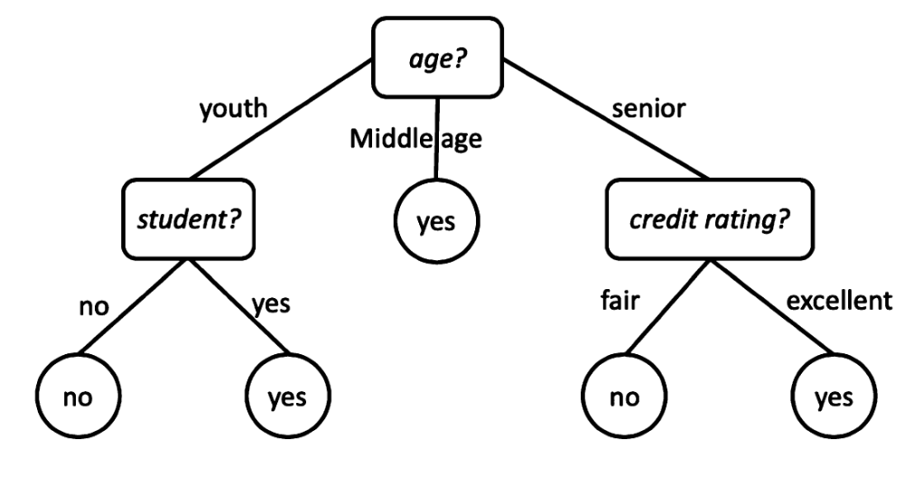
• a decision tree is flowchart-like structure
  • each internal node represents a test on an attribute
  • each branch corresponds to an outcome of that test
  • each leaf node contains a class label

root도 leaf도 아닌 node를 internal node라 한다.

• how decision trees perform classification
  • to classify a new instance
  • we start at the root node
  • evaluate the test condition at each node
  • follow the corresponding branch based on the feature values
  • continue this process until reaching a leaf node
• the label stored in the leaf node is the predicted class
  • classification is essentially a path traversal from root to leaf

2.3 Representative Algorithms

ID3

• iterative dichotomiser 3
• uses information gain for splitting
• handles categorical attributes only
• dose not perform pruning

C4.5

• extension of ID3
• supports continous attributes
• uses gain ratio
• includes post-pruning

편향을 줄이기 위해 gain ratio를 사용한다.

CART(Classification and Regression Trees)

• generate binary trees only
• supports both classification and regression
• uses gini index for classification, and MSE/RSS for regression

Common Characteristics

• uses greedy strategy
• constructs trees in a top-down recursive manner
• aims to produce pure paritions at each node

2.4 Basic Algorithm

Supervisesd Learning이므로 $y$, 정답에 해당하는 클래스 라벨이 포함된 학습용 데이터셋을 사용한다.

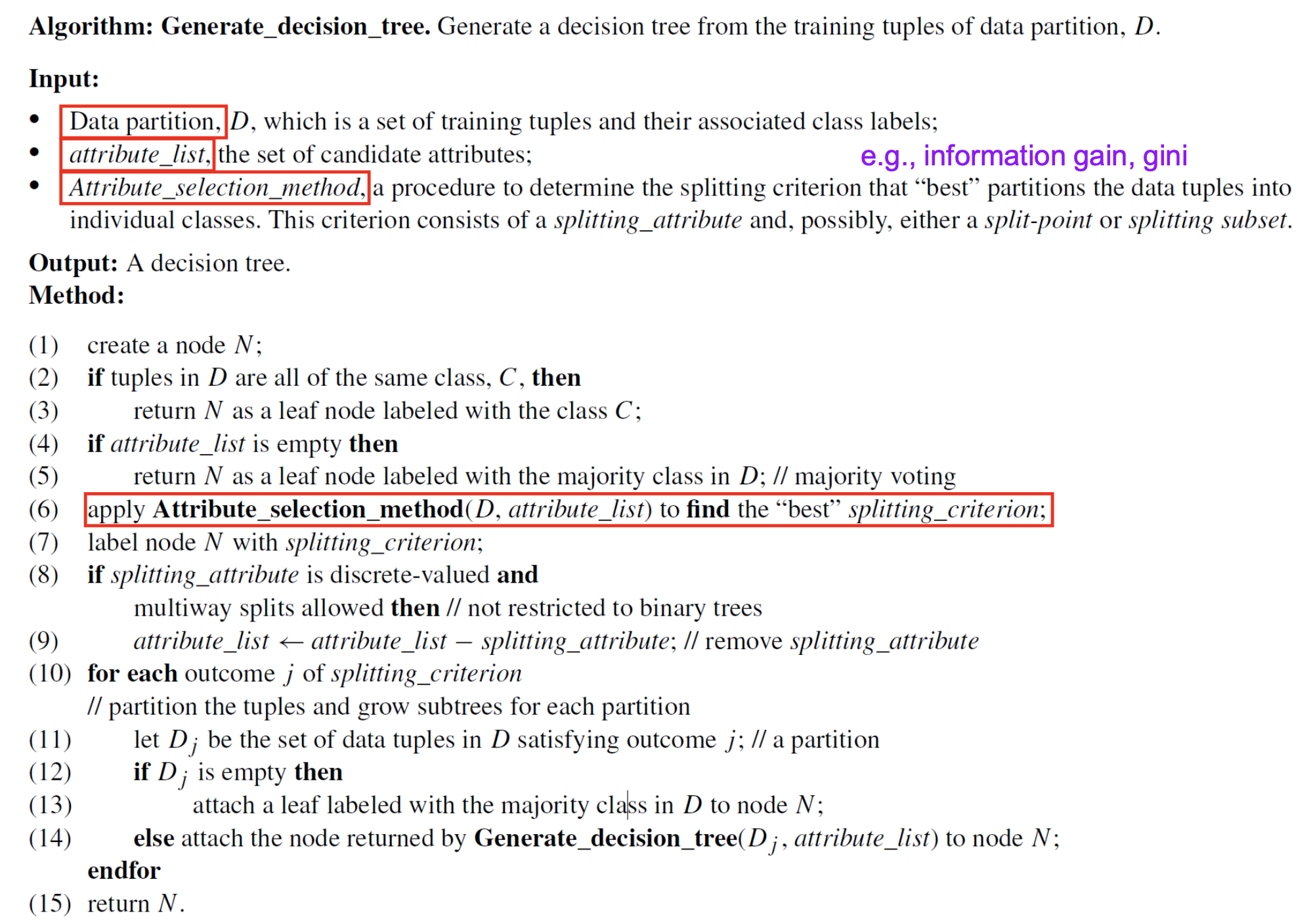
• 노드 생성
• 종료 조건 (1): 모든 항목이 이미 같은 정답이라면
• 종료 조건 (2): 더 이상 나눌 기준이 남아있지 않다면, 다수결 원칙에 따라 가장 많은 항목이 속한 클래스를 정답으로 선택
• 최선의 기준 찾기
• 가지치기: 선택된 기준에 따라 하위 그룹으로 분할
• 재귀적 반복

모든 가지가 리프 노드에 도달할 때까지 하향식 재귀 방식으로 반복된다. 속성이 남아있지 않은 경우, 데이터가 혼합된 상태일지라도 다수결 원칙을 적용하여 가장 우세한 클래스로 최종 결론을 내린다.

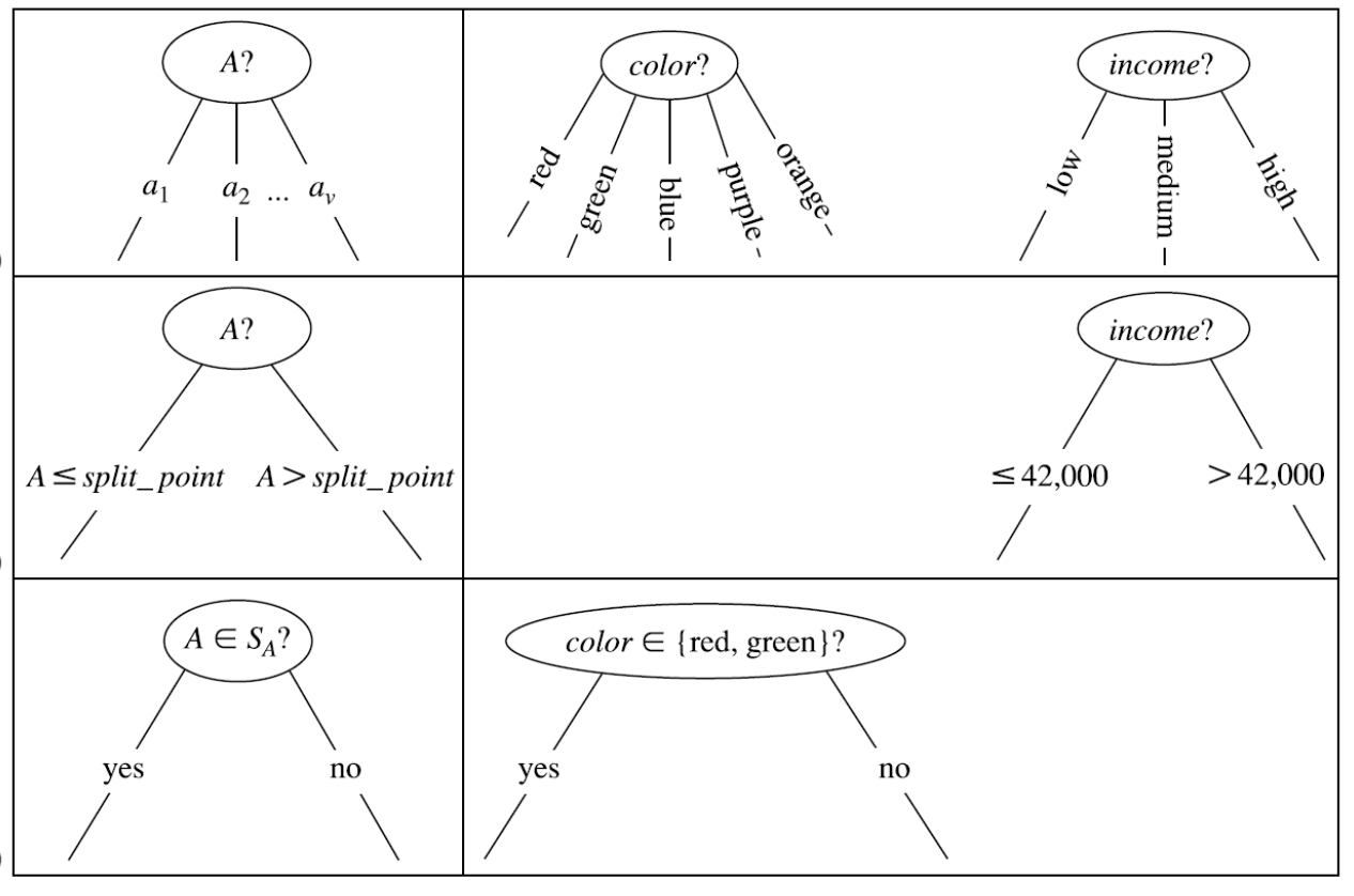
2.5 Partitioning

1. discrete attribute
   • multi-way split
2. continous attribute
   • threshold split
3. binary split on discrete attribute

2.6 Attribute Selection Measures

• a heuristic used to select the best splitting attribute at each node
• determines how the dataset is partitioned into smaller subsets

objective

• create subsets that are as pure(homogeneous) as possible
• a pure node contains tuples from only one class

pure하게 만든다는 것은 서로 다른 것들이 섞이지 않은 동질적인 상태로 만드는 것과 같은 의미이다.

1. Entropy

• $Info(D) = - \sum ^m_{i=1} p_i log_2 (p_i)$
  • 단, $p_i = \frac{|C_{i, D}|}{|D|}$; $D$에서 각 클래스 $i$가 차지하는 비율
• impurity of the dataset $D$

2. Information Gain (ID3)

• $Gain(A) = Info(D) - Info_A(D)$
  • $Info_A(D) = \sum ^v_{j=1} \frac{|D_j|}{|D|} \times Info (D_j)$; 속성 $A$로 분할한 후의 기대 정보량
• how much uncertainty is reduced after splitting
• selects attributes with maximum gain

특정 속성 $A$로 데이터를 나누었을 때 불확실성이 얼마나 감소하는지 측정한다. 원래의 엔트로피에서 분할 후의 엔트로피를 뺀다.

3. Gain Ratio (C4.5)

• $GainRatio(A) = \frac{Gain(A)}{SplitInfo_A(D)}$
  • $SplitInfo_A(D) = - \sum^v_{j=1}\frac{|D_j|}{|D|} \times log_2(\frac{|D_j|}{|D|} )$
• nomalized version of information gain
• reduces bias toward attributes with many values

정보 이득이 값이 많은 속성을 선호하는 편향을 해결하기 위해 정규화한 지표이다. 속성이 얼마나 잘게 쪼개지는지를 분모로 두어 벌점을 준다.

4. Gini Index (CART)

• $Gini(D) = 1 - \sum^m_{i=1} p^2_i$
  • 단, $p_i = \frac{|C_{i, D}|}{|D|}$
• measures the impurity of a dataset

모든 데이터가 하나의 클래스에 속해 있다면 지니 지수는 0(최소 불순도)이다. CART 알고리즘은 오직 이진 트리만을 생성하며 이 지수가 가장 낮은 방향으로 가지친다.

Entropy vs. Gini Index

구분	Entropy	Gini Index
주요 알고리즘	ID3, C4.5	CART
수식	$Info(D) = -\sum_{i=1}^{m} p_i \log_2(p_i)$	$Gini(D) = 1 - \sum_{i=1}^{m} p_i^2$
트리 구조	다중 분할 가능	이진 트리만
계산 효율성	로그 계산으로 상대적으로 느림	제곱 합 계산으로 연산 속도 빠름
주요 목표	불확실성의 최소화 및 정보 이득 최대화	데이터셋의 불순도 측정 및 최소화

---

3. Information Gain

3.1 Information Gain

1. compute entropy of $D$
2. partition by attribute
3. compute entropy for each partition
4. compute conditional entropy
5. compute information gain

the attribute with the highest information gain is selected, and pure partitions directly becomes leaf nodes

3.2 Gain Ratio

Limitation of Information Gain

• bias toward many-valued attributes
• information gain prefers attributes with many distinct values
  • each value a seperate partition, each partition contains one tuple
  • entropy = 0, gain = info(D) - 0 $\rightarrow$ maximum

Split Information

• measures how evenly data is split
• similar to entropy, but not class-based

Gain Ratio

• overcome bias of information gain
  • information gain normalized by how evenly data is split
• better generalization than pure information gain

3.3 Gain Impurity

Gini Impurity

• measures the impurity of dataset $D$

Interpretation

• gini = 0 $\rightarrow$ completely pure (all same class)
• gini $\uparrow$ $\rightarrow$ more mixed classes

Binary splitting in CART

• e.g., low vs. medium, high 4

Process

1. compute the gini impurity of the dataset
2. try a binary split on the attribute
3. compute the weighted gini after the split
4. interpretation

지니 불순도는 데이터셋에서 임의로 선택한 요소에 임의로 라벨을 지정했을 때, 얼마나 자주 틀릴지를 수치화한 것이다. 즉 데이터가 얼마나 섞여 있는지를 보여주는 지표이다.