1. Decision Tree Pruning
why do we need pruning?
- overfitting
- complex
- poor performance on unseen data
a very detailed tree memorizes the training data, but fails to generalize
pruning makes the tree smaller, easier to interpret, faster, more accurate on test data
1.1 Approaches
Pre-pruning
- stop splitting during tree construction
- use criteria
- e.g., Information Gain, Gini
- node becomes a leaf if split is not significant
- risk: underfitting
트리가 완전히 만들어지기 전, 트리 구축 중에 분할을 중단한다. 분할이 멈춘 노드는 즉시 리프 노드가 된다.
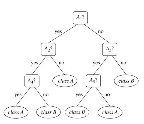
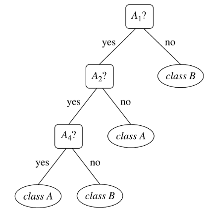
Post-pruning (backward pruning)
- build full tree first
- remove unnecessary subtrees
- replace subtree with a leaf (majority class)
- more reliable but computationally expensive
전체 트리를 다 만든 후에 불필요한 부분을 제거해 나가는 방식으로 비싸다.
Key Idea
balance between model complexity and generalization
1.2 Representative Methods
1. Cost Complexity Pruning (CART)
- minizes a cost function that combines error rate and tree complexity
- compare subtree vs. pruned version to select with lower cost
- a pruning dataset is typically used to choose the optimal complexity parameter
가 0이면 페널티가 없어 복잡한 트리가 되고 가 커지면 페널티가 커져 에러가 조금 늘어나더라도 단순한 트리를 선택한다. 위 식을 통해 모델의 복잡도와 일반화 성능 사이의 균형을 맞출 수 있다.
2. Pessimistic Pruning (C4.5)
- uses only training data (no pruning set)
- adds a penalty to obtain a more realistic error estimate
- subtrees are pruned if the corrected leaf error is lower than the subtree error
훈련 데이터에 과적합을 경계하여 에러가 더 많이 날 것이라고 보수적으로 가정하고 트리를 단순화한다.
3. MDL-based pruning
- select the model that minimizes total encoding length
- balances model complexity and data fitting by considering both tree size and precision errors
- subtrees are pruned if replacing them with a leaf reduces the overall description length
트리 크기에 대한 비용과 에러 비용을 모두 길이 단위로 환산하여 최적의 모델을 찾는다.
1.3 Model Evaluation and Selection
- after building a classifier, we must ask
- how accurate is our model?
- will it generalize to unseen data?
- how do we compare multiple models?
- training accuracy is often overly optimistic due to overfitting
- evaluation must be done on unseen test data
1.4 Confusion Matrix and Metrics
Confusion matrix
- TP: correctly predicted positivies
- TN: correctly predicted negatives
- FP: false alarms
- FN: missed positives
Metrics
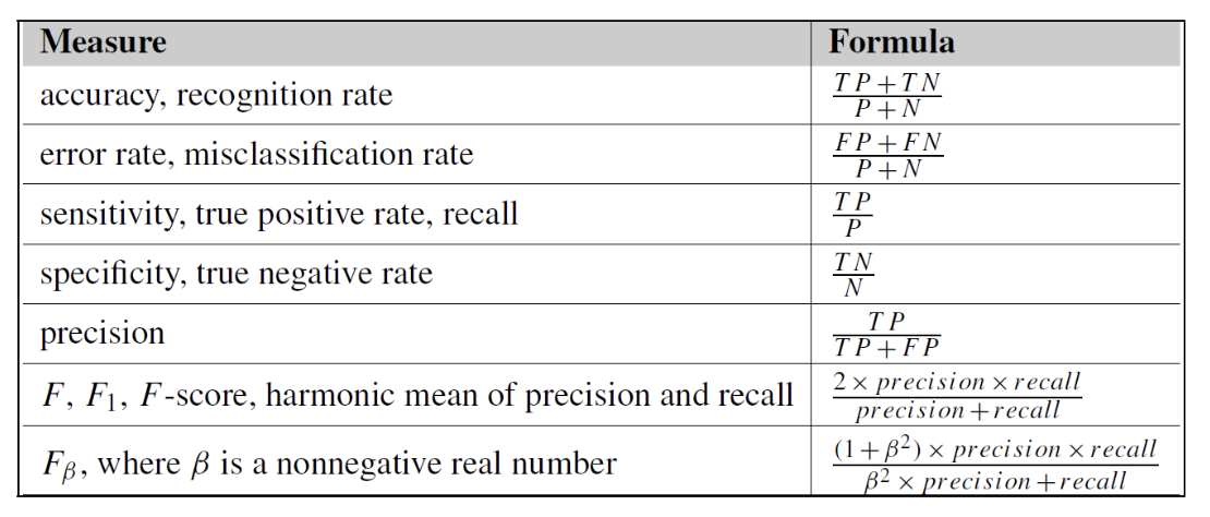
each metric provides different perspectives on model performance
1.5 Limitation on Accuracy
Class Imbalance
- in real-word, the positive class is rare, while the negative class dominates the dataset
- a model can achieve high accuracy by predicting only the majority class
Problem
- the model ignores the minority (but often important) class in critical applications such as medical diagnosis or security
- and missing positive cases (false negatives) can be very costly
Solution
- use evaluation metrics that focus on the positive class
- precision: reliability of positive predictions
- recall(sensitivity): ability to detect positives (rare class)
- F1-score: balance between precision and recall
1.6 Reliable Evaluation Methods
1. Holdout
- split data into training set and test set
- simple and fast, results may very depending on the split
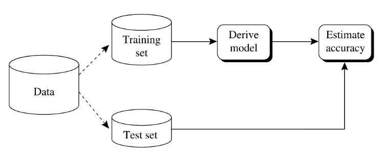
데이터를 2개로 쪼개든 3개로 쪼개든, 한 번 정해진 분할을 고정해서 사용한다.
2. Cross-Validation
- divide data into multiple folds
- train and test repeatdly on different splits
- provides more stable and reliable esimates
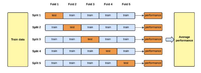
데이터를 여러 번 다시 나누어 평가하기 때문에 더 안정적이고 신뢰할 수 있는 추정치를 제공한다.
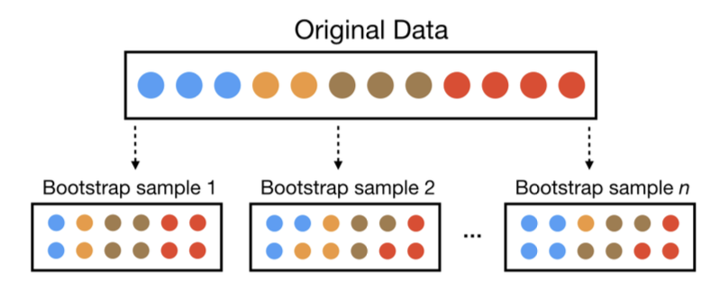
3. Bootstrap
- sample data with replacement
- evaluate performance across multiple resampled datasets
- useful when data is limited
Goal
- obtain a reliable estimate of generalization performance
- reduce bias and variance in evaluation
- ensure fair comparison between different models
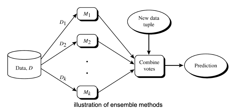
2. Ensemble
2.1 Ensemble Learning
- ensemble methods combine multiple models
- each classifier "votes" for the class label of the given data
- to build a strong composite model and improve classification performance
Process
- generate multiple training set
- train base classifiers
- each model produces a prediction
- final prediction is based on combined outputs
2.2 Voting Mechanism
- each classifier outputs a class label ("votes")
- final prediction
- (classification) majority voting
- (regression) averaging
- improved accuracy through diversity
- ensemble makes an error only when the majority of models are wrong
- more robust and stable than a single model
- low correlation between models
- if all models are highly similar, they tend to make the same mistake
- if models are less correlated, errors are less likely to overlap
모델이 서로 다른 방식으로 학습하면 실수를 하더라도 서로 다른 지점에서 하게 된다.
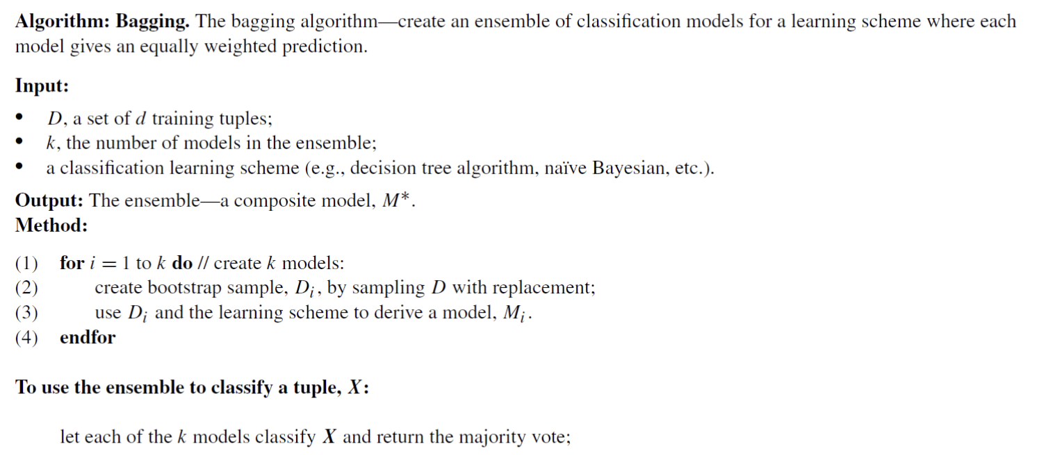
2.3 Bagging
- given a dataset with samples:
- we create multiple training sets
- each dataset is generated using bootstrap sampling (w/ replacement)
- some samples may appear multiple times, while some samples may not appear at all
Training Process
- for each iteration
- sample dataset from (w/ replacement)
- train a model using
- we obtain multiple models
Prediction Process
- given a new data sample
- each model independently makes a prediction
- each prediction is treated as one vote
- final output
- (classification) the class with the highest number of votes is selected majority voting
- (regression) the final output is the average of all predictions
Why Bagging Works
- reducing variance
- stabilizing predictions through averaging
- averaging multiple models reduces fluctuations in predictions
- handling noise and overfitting
- different training samples produce different models
- and the effect of noise is reduced through aggregation
2.4 Boosting
- assign different weights to each doctor based on past performance
- focus more on hard(misclassified) samples and gradually improves performance
Mechanism
- boosting build models sequentially
- models are trained one after another
- each new model focuses on correcting previous errors
Process
- initialize all training samples with equal weights
- train the first model
- increase weights of misclassified samples
- train the next model focusing more on difficult samples
- repeat for rounds
model progressively focuses on harder examples
2.5 AdaBoost
Boosting 기법을 구현한 대표적인 알고리즘이다.
Initialization
- assign equal weight to each training sample
- : data
Iterative Learning
- for each round
1. sample data according to weights- train model
- compute error of
Weight Update
- misclssified samples increase weights
- correctly classified samples decrease weights
Model Combination
- each model contributes with a different weight
- models with lower error receive higher weight
Prediction Process
- given a new data sample :
- each model makes a prediction
- each prediction is weighted
- the class with the highest weighted vote is selected
Why Boosting Works
- focues on difficult samples
- models complement each other different models correct different mistakes
- reduces bias model can better capture complex patterns
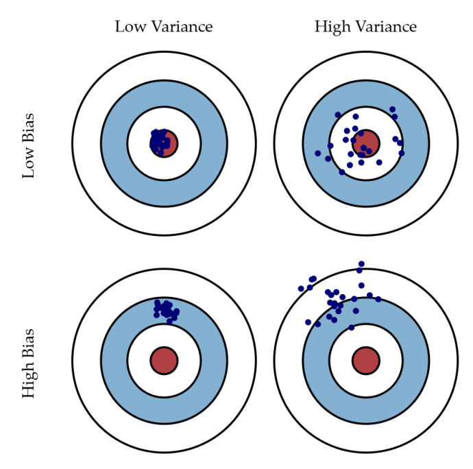
머신러닝의 궁극적 목표는 편향과 분산을 모두 낮추어 일반화 성능을 극대화하는 것이다.
- Boosting은 모델들이 서로의 실수를 보완하므로 정답에 쏠려 있던 편향을 직접적으로 낮추는 효과가 있다.
- Bagging은 모델을 병렬 학습시키기 때문에 개별 모델이 가진 근본적인 편향 자체를 수정하지는 못하고 주로 분산을 줄이는 데에 효과적이다.
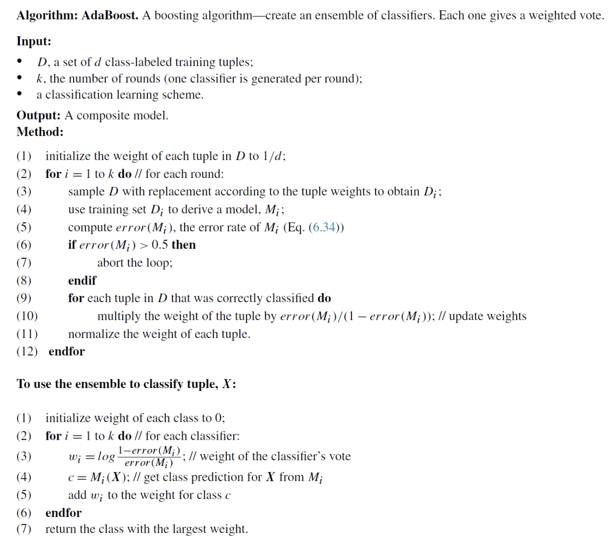
- 에러율이 작을수록: 분모인 가 작아지므로 로그 안 값이 매우 커져 가중치도 커진다. 즉 성능이 좋은 모델에게 훨씬 강력한 투표권을 준다.
- 에러율이 0.5(무작위 추측)에 가까울수록: 로그 안의 값이 1에 가까워져 는 0에 수렴한다. 쓸모 없는 모델의 의견은 반영하지 않는다.
를 계산할 때 log 함수로 모델의 에러율에 따라 성능이 높은 모델에는 확실한 보상을 주고, 낮은 모델은 무시한다.
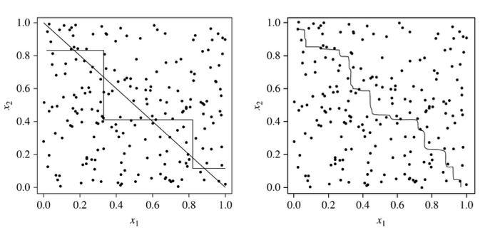
2.6 Random Forest
a collection of trees is called a "forest"
- a single decision tree tends to be unstable and has high variance
- multiple trees produce more stable and accurate predictions
- build many decision trees using randomness
- combine their predictions for better performance
Basic Mechanism
- bagging (bootstrap sampling)
- generate multiple datasets
- each dataset is sampled with replacement
- random feature selection
- at each split, randomly select a subset of features
- not all features are used at every node
데이터를 무작위로 뽑고 특징도 무작위로 선택하여 수많은 나무를 만든다. 개별 나무들 사이의 상관관계가 낮아져 전체적인 예측 성능과 정확도가 단일 트리보다 훨씬 뛰어나다.
Training Process
- for each tree
- create a bootstrap sample
- train a decision tree
- at each node
- randomly select features
- choose the best split among the selected features
각 노드에서 나무가 뻗어 나가는 기준이 매번 무작위로 결정되며 나무를 심기 전 단계에서도 부트스트랩 샘플링을 통해 랜덤성이 적용된다.
Prediction Process
- given a new sample
- each tree makes a prediction
- final output
- (classification) majority voting
- (regression) averaging