5. Linear Model (1)

1. Linear Model

1.1 Making a Decision

to make a decision

• weighted coordinates are combined to form a 'credit score'
• the resulting score is then compared to a threshold value

E.g., Credit Approval

• for input $x = (x_1, ..., x_d)$, attributes of a customer
• approve credit if $\sum_{i=1}^{d} w_i x_i > \text{threshold}$
• deny credit if $\sum_{i=1}^{d} w_i x_i < \text{threshold}$

데이터의 각 속성을 선형 결합하여 데이터를 어떻게 나눌 것인지(결정경계) 결정하는 최적의 가중치를 찾는 것이 학습의 목적이다.

1.2 Perceptron

위에서 언급된 의사결정 수식을 더 간결하게 표현한 가설 집합 $h \in \mathcal{H}$를 Perceptron이라 부른다.

$h(x) = \text{sign}\left((\sum_{i=1}^{d} w_i x_i) - \text{threshold}\right)$
$=\text{sign}\left((\sum_{i=1}^{d} w_i x_i) + b\right)$

• $b$(bias): 기존의 임계값을 수식 안으로 포함시킨 값
• $sign$: 입력값이 0보다 크면 +1, 작으면 -1 반환
  • 이진 분류를 수행하는 계단 함수 역할

1.3 Two-dimensional Case

Plane

• the plane is split by a line into two regions
  • +1 decision region(blue) and -1 decision regin(red)

Decision Boundary

• different values for parameters $w_1, w_2, b$
  • corresppond to different lines $w_1x_1 + w_2x_2 + b = 0$

Vector Form

• for simplification, treat bias $b$ as weight $w_0 = b$
• introduce an artificial coordinate $x_0 = 1$
• with this convention, $w^Tx = \sum_{i=0}^{d} w_i x_i$
  • this yields the perceptron in vector form

$h(x) = sign(w^Tx)$

단일 퍼셉트론으로 데이터가 직선으로 완벽히 나눠질 수 있다는 Linearly Separable 가정을 전제로 한다.

---

2. The Framework of Learning

2.1 Roles of the Learning Algorithm

Search $\mathcal{H}$

• by looking for weights and bias that perform well on data set

가설 집합 $\mathcal{H}$은 학습 알고리즘이 탐색할 수 있는 모든 가능한 후보 모델들의 모임이다.

Produce the final hypothesis $\mathcal{g} \in \mathcal{H}$

• $\mathcal{g}$ is defined by the optimal choice of weights and bias

실제 환경의 target function $f$는 접근할 수 없다. 따라서 학습 알고리즘이 $\mathcal{H}$이라는 후보 중 데이터셋을 참고하여 가장 성능이 좋은 최종 가설 $\mathcal{g}$를 하나 선택한다.

2.2 Three Important Problems in Linear Models

1. Classification

2. Regression

3. Probability Esitmation

• a.k.a logistic regression
• come with different but related algorithms

분류는 sign을 쓰고, 회귀는 제곱 오차를 최소화한다. 로지스틱 회귀는 확률을 가장 잘 설명하는 가중치를 찾기 위해 또 다른 최적화 알고리즘을 사용한다.

2.3 Generalization and Complexity

Set of lines

• often a good first choice

VC dimension

• 학습 모델이 가질 수 있는 용량, 표현할 수 있는 복잡도를 나타내는 척도

선형 모델은 상대적으로 낮은 VC 차원을 가진다.

From $E_{in}$ to $E_{out}$

• generalize well from $E_{in}$ to $E_{out}$
• $E_{in}$: 가지고 있는 학습 데이터 내에서 발생하는 오류
• $E_{out}$: 학습에 사용되지 않는 새로운 데이터에서 발생하는 오류, 모델의 실제 성능

선형 모델처럼 VC 차원이 낮으면 학습 데이터에서 얻은 성능과 실제 데이터에서의 성능의 차이가 크지 않다. 데이터 분석을 처음 시작할 때 복잡한 모델을 바로 쓰면 일반화에 실패할 확률이 높기에 선형 모델을 종종 사용한다.

---

3. Perceptron Learning Algorithm

3.1 Objective and Fundamental Assumption

Objective

• determine the optimal $\mathbf{w}$ based on the data to produce $\mathcal{g}$

Assumption

• the data set is linearly separable
• there is a vector $\mathbf{w}$ that makes $h(x) = sign(\mathbf{w^Tx})$ achieve the correct decision $h(\mathbf{x}_n) = y_n$ on all training examples

3.2 How PLA Works

• an iterative algorithm
• guaranteed to converge for linealy separable data

1. Initialize

• 학습 데이터셋 $(\mathbf{x}_1, y_1), (\mathbf{x}_2, y_2), \dots, (\mathbf{x}_N, y_N)$
• 초기 가중치 벡터 $\mathbf{w}(0)$로 학습 시작
• 퍼셉트론은 $h(x) = \text{sign}(\mathbf{w}^T\mathbf{x})$ 형태의 가설 구현

2. Pick a Misclassified Point

• 매 반복마다 데이터셋에서 샘플 포인트 하나씩 확인
• $y_n \neq \text{sign}(\mathbf{w}^T\mathbf{x}_n)$인 오분류 지점 하나 선택

PLA는 한 번에 하나의 데이터를 확인하며 가중치를 수정하는 반복적 알고리즘이다.

3. Updata Rule

• 선택된 오분류 데이터를 바탕으로 가중치 벡터 업데이트
• 실제 값 $y_n$이 $+1$이면 벡터를 더하고, $-1$이면 벡터를 빼는 방식으로 조정

4. Geometric Effect

• 결정 경계를 오분류된 $\mathbf{x}_n$을 올바르게 분류할 수 있는 방향으로 이동
• 가중치 벡터에 $y_n\mathbf{x}_n$을 더함으로써 경계의 각도를 틀어 데이터가 올바른 영역에 속하도록 함

5. Convergence

• Termination Condition
  • 데이터셋 내 더 이상 오분류된 예시가 없을 때까지 반복
• Convergence Guarantee
  • 데이터셋이 선형 분리 가능하다면, PLA는 유한한 횟수 내 반드시 수렴하여 모든 데이터를 완벽히 분류하는 최적의 $\mathbf{w}$를 찾는다.

---

4. Non-linearly Separable Data

4.1 Linear Model for Binary Classification

• uses a hypothesis set of linear classifiers
  • each $h$ has the from

$h(x) = sign(w^Tx)$

• $w \in \R^{d+1}$: weight column vector
• $d$: input dimension
• $x_0=1$: corresponds to bias $w_0$
  • $w_0$(bias)를 계산식에 포함시키기 위해 넣은 상수

$w^Tx$: 입력 벡터 $x$와 가중치 벡터 $w$의 선형 결합을 의미하며 signal이라 부른다. 수학적으로는 $w_0x_0 + ... + w_dx_d$와 같이 계산된다.
$sign()$: 괄호 안의 값이 양수이면 +1, 음수이면 -1을 출력한다. 출력을 통해 최종적으로 데이터를 두 개의 카테고리 중 하나로 분류한다.

• we use $h$ and $w$ interchangeably to refer to the hypothesis
• PLA finds an optimal $w$ for linearly seperable data

4.2 Non-linearly separable

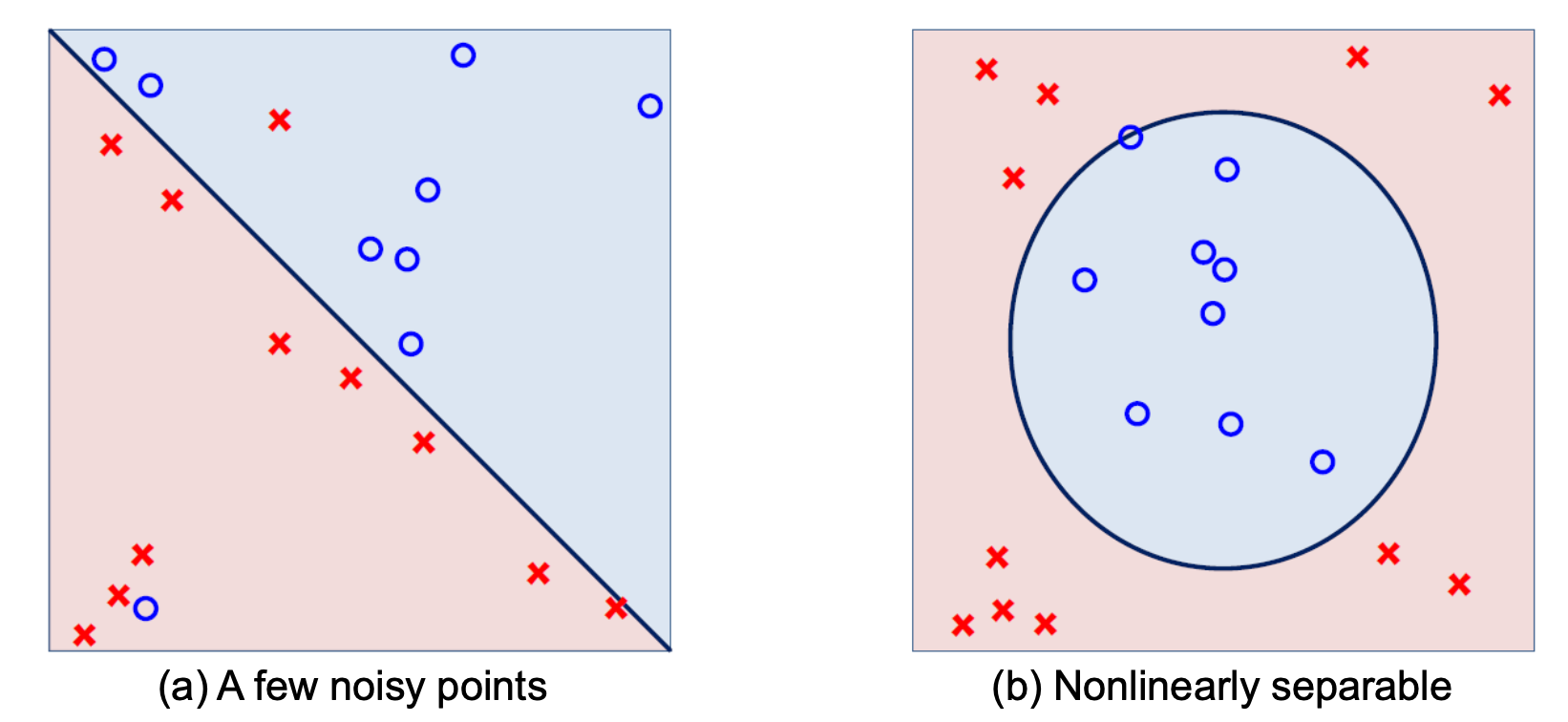
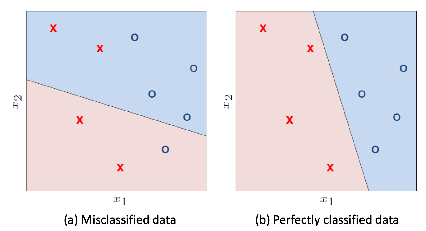
a: a few noisy points

• it seems appropriate to stick with a line
• but to somehow tolerate noise
• and output a hypothesis with a small $E_{in}$

데이터가 조금 지저분해도 직선 모델의 단순함을 믿고 완벽(0)보다는 최선(small $E _{in}$)의 결과물을 찾는다.

b: a circle rather than a line

• the linear model does ot seem to be correct
• may need a technique called nonlinear trnasformation

4.3 Hardness of Minimizing $E_{in}$

• the situation in (a): encountered very often in practice
  • a linear classifier seems appropriate
  • but data may not be linearly separable due to outliers/noise
• to find a hypothesis with the minimum $E_{in}$
  • need to solve combinatorial optimization

$\displaystyle \min_{\mathbf{w} \in \mathbb{R}^{d+1}} \frac{1}{N} \sum_{n=1}^{N} \left[ \text{sign}(\mathbf{w}^T \mathbf{x}_n) \neq y_n \right]$

• equation: difficult to solve
  • in general, NP-hard (there is no known efficient algorithm for it)
  • due to the discrete nature of both $sign(\cdot)$ and $[\cdot]$
    $\rightarrow$ approximately minimize $E_{in}$

---

5. The Pocket Algorithm

5.1 Approximately Minimizing $E_{in}$

완벽한 최소값 대신 최대한 근사적으로 $E_{in}$을 최소화하는 전략을 취하며 이를 위해 PLA를 수정한 Pocket Algorithm을 도입한다.

• extend PLA through a simple modification
• pocket algorithm with ratchet

마치 한쪽 방향으로만 회전하는 라쳇 렌치처럼 알고리즘은 지금까지 발견한 가장 좋은 가중치를 유지하며 더 나쁜 결과로 퇴보하지 않도록 설계되었다.

5.2 Algorithm

• the pocket algorithm keeps 'in its pocket' the best $\mathbf{w}$ encountered up to iteration $t$ in PLA
• at the end, the best $\mathbf{w}$ will be reported as the final hypothesis

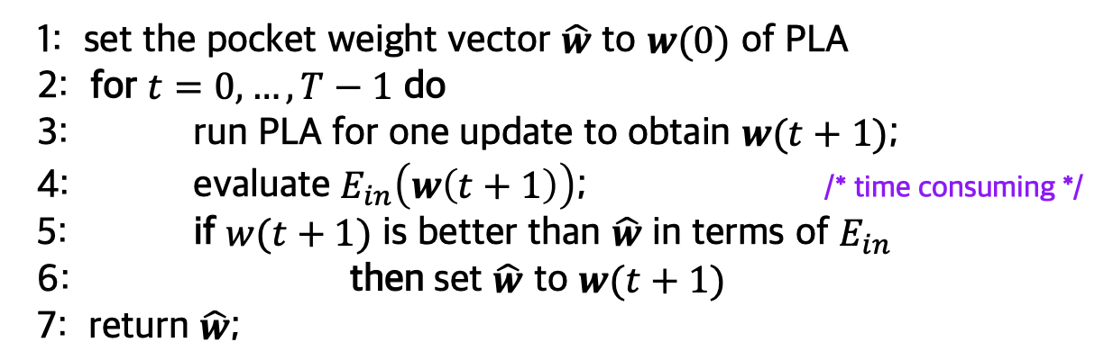
• line4: evaluate all examples to get $E_{in}(\mathbf{w}_{t+1 })$
  • much slower than PLA

PLA는 선형 분리 불가능한 데이터에서 $E_{in}$이 계속 요동치지만 Pocket Algorithm은 지금까지 중 최고를 보관하므로 반복 횟수가 늘어남에 따라 $E_{in}$과 $E_{out}$이 안정적으로 감소한다.

---

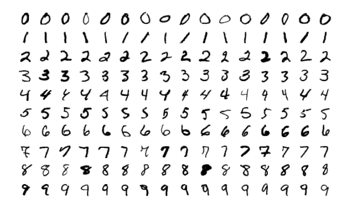
6. Handwritten Digit Recognition

• data: sampled digits from the US Postal Service zip code DB
  • each image has 16 $\times$ pixels

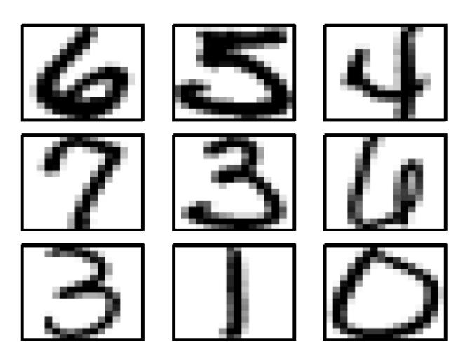
• goal: recognize each digit
  • non-trivial task (even human $E_{out}$ is about 2.5%)
  • common confusion: digits {4, 9} and {2, 7}

6.1 Solution Components

1. Decomposition

• from multiclass to binary classification
• a commonly used approach for multiclass setup

2. Feature Extraction

• a human approach to determining the digit of an image
  • look at the shape (or other properties) of black pixels
• rather than carrying all the info in 256 pixels, summarize the info contained in the image into a few features
• again a very common/essntial approach in machine learning

E.g., focus on digit {1, 5}

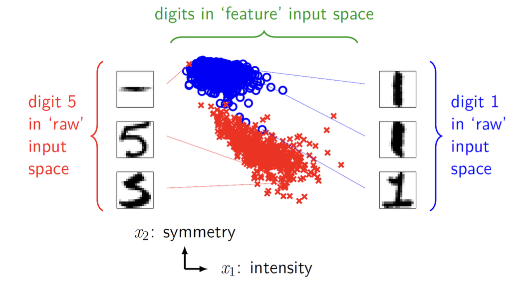
• a scatter plot for these intensity and symmetry features
  • $\mathbf{x} = (x_0, x_1, x_2)$
• observation
  • digit 5 usually occupies more black pixels than digit 1
  • digit 1 is symmetric while digit 5 is not

6.2 Performance Evaluation

Feature space에서 PLA와 Pocket 알고리즘을 적용하여 성능을 비교하였다.

Error vs. Iteration

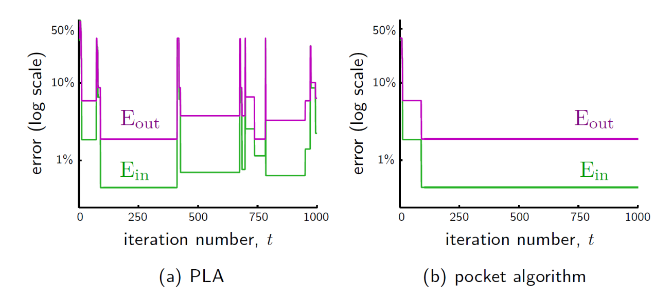
• PLA
  • 반복 횟수가 늘어남에 따라 오류율 크게 요동침
  • 1,000번 반복 후 $E_{in}$ = 2.24% $E_{out}$ = 6.37%
• Pocket Algorithm
  • 가장 좋은 결과를 보존하는 특성 덕분에 오류율 안정적으로 낮게 유지
  • 1,000번 반복 후 $E_{in}$ = 0.45%, $E_{out}$ = 1.89%로 PLA보다 월등한 성능

Learned Hypothesis $\mathcal{g}$

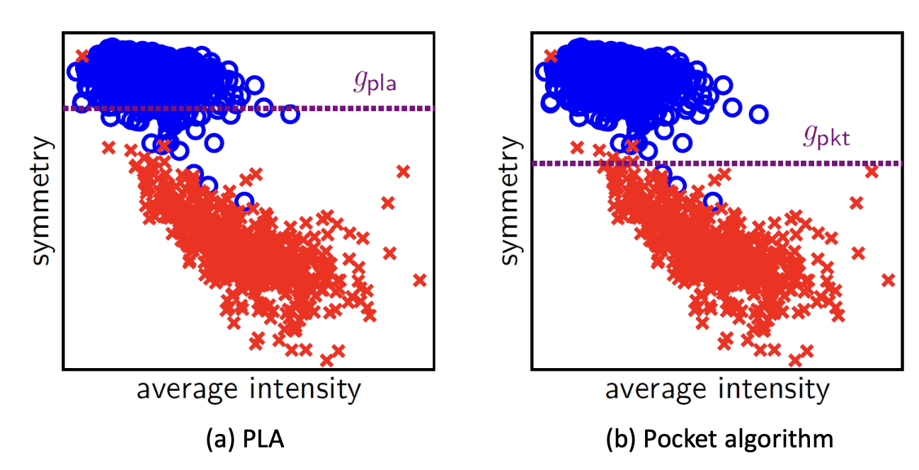
Pocket 알고리즘을 통해 얻은 결정 경계 $\mathcal{g}_{pkt}$가 PLA$\mathcal{g}_{pla}$보다 데이터 군집을 훨씬 더 정확하게 가로지르며 분리해 내는 것을 확일할 수 있다.

MNIST Dataset

더 방대한 MNIST 데이터셋(70k digits)에 대해 다양한 모델의 오류율을 비교한 결과이다.

• Linear Model: 7.6%
• Gaussian SVM: 1.4%
• CNN: 0.23%

이 데이터셋은 제프리 힌튼에 의해 머신러닝의 초파리라고 불릴 만큼 연구의 기본 모델로 활용된다.