1. Matrix Representation: Data and Error
1.1 Data Matrix and Target Vector
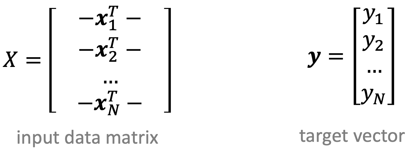
Data Matrix
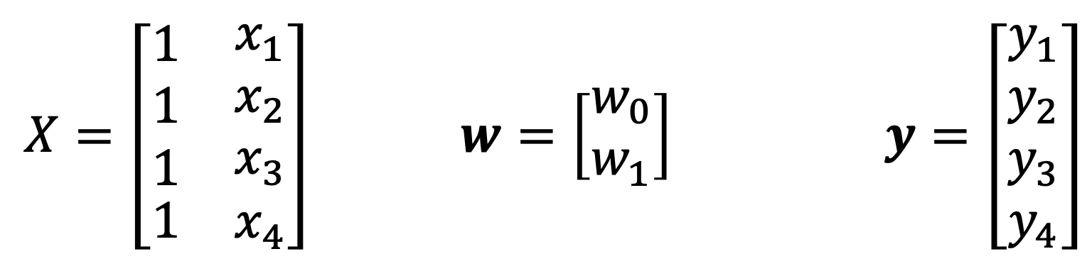
- X∈RN×(d+1)
- rows: inputs xn as row vectors
각 개별 데이터 벡터xn에 1(bias coordinate)이라는 항목을 추가한 뒤, 데이터 행렬 X를 만들 때는 개별 벡터들을 행 벡터 형태인 xnT로 변환하여 차례대로 쌓는다.
Target Vector
- y∈RN
- components: target values yn
타겟 벡터 y의 n번째 요소인 yn은 데이터 행렬 X의 n번째 행 xnT에 1:1로 대응되는 실제 결과값을 의미한다.
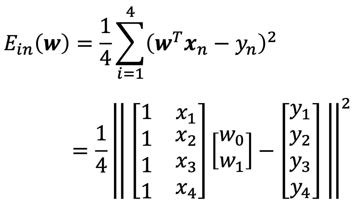
E.g., d = 1, N = 4
In-sample Error
- A function of w and data X, y
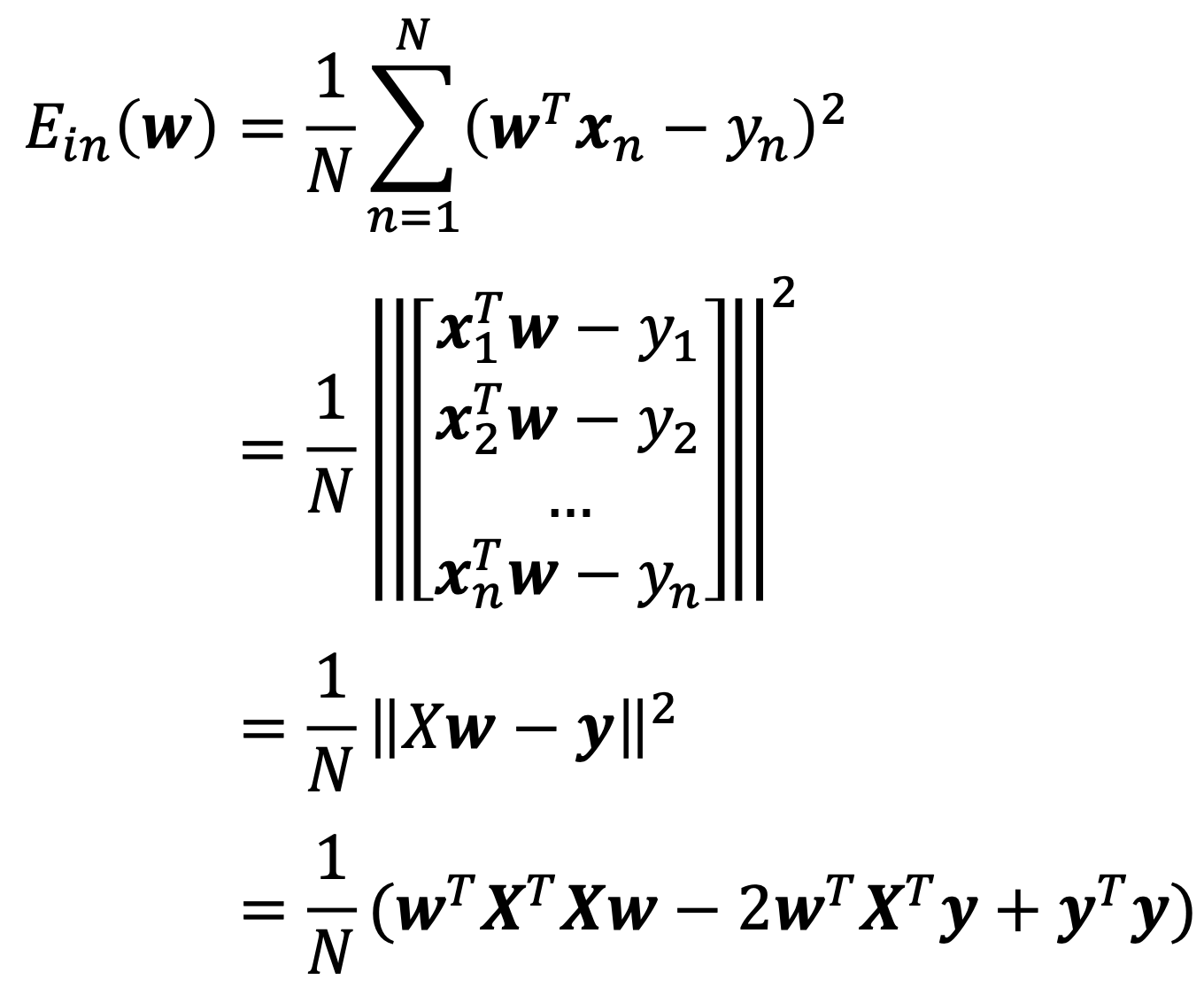
- ∣∣⋅∣∣: Eculidean norm of a vector
- Scalar yTXw=(wTXTy)T=wTXTy
학습 오차 Ein를 행렬 형태로 표현하는 것은 수만 개의 데이터를 하나씩 계산하지 않고 한 번의 행렬 연산으로 전체 오차를 정의하기 위함이다.
- 합산 형식에서 행렬 형식으로의 변환
- 예측값 벡터 Xw, 잔차 벡터 Xw−y
- 행렬식의 전개 과정
- 벡터의 2-norm은 a2=aTa
- 스칼라 성질을 이용한 단순화
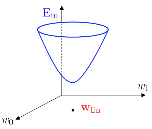
정리하면 2차 함수 형태, 미분 가능하며 볼록한 모양을 가진다. 이는 기울기가 0인 지점을 찾았을 때 그곳이 반드시 최솟값임을 보장한다.
E.g., d = 1, N = 4
2. Getting the Solution wlin
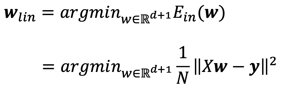
5.1 Minimization of Ein(w)
wlin
- The solution to linear regression
- Derived by minimizing Ein(w) over all possible w∈Rd+1
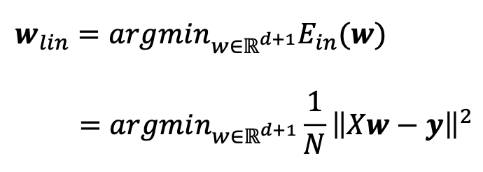
- 모든 데이터의 예측값 Xw과 실제 정답 y의 차이를 구함 → 잔차
- 잔차의 제곱합을 평균 내어 전체 오차 Ein을 구함
- Ein이 가장 낮아지는 지점의 가중치 wlin을 찾음
Ein(w) is continous, differentiable, and convex
- Convexity: 함수 그래프 위의 임의의 두점을 연결했을 때, 그 선분이 함수 공간을 빠져나가지 않는 형태
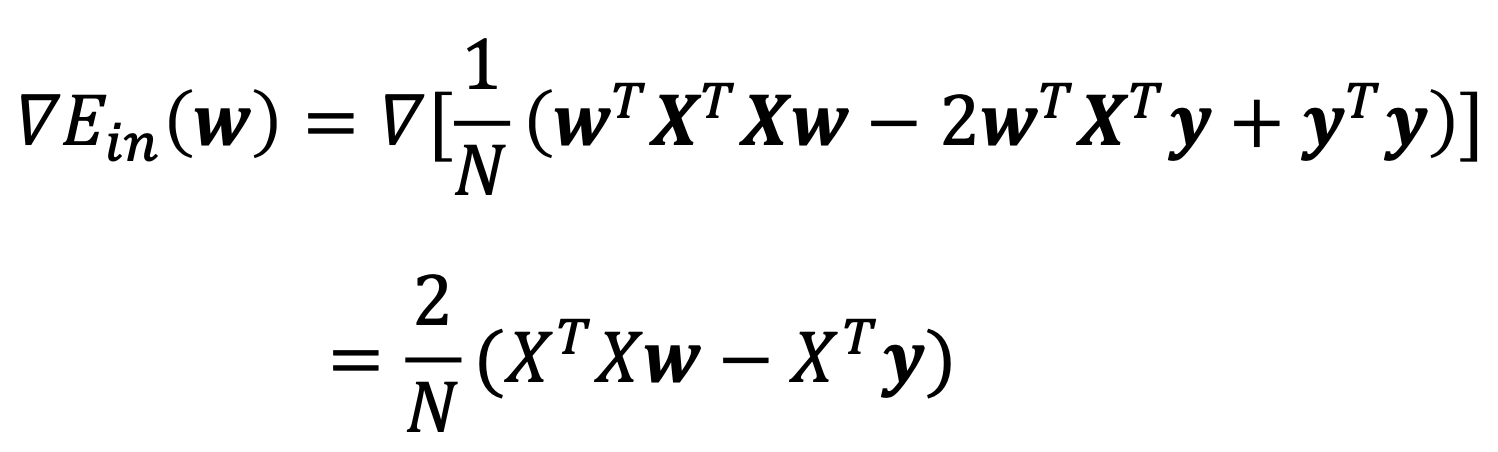
Ein(w)=N1(wTXTXw−2wTXTy+yTy)
- We can use standard matrix calculus to find w that minimizes Ein(w) by requiring
- ∇Ein(w)=0
- General optimization techniques
Gradient Identities
∇w(wTAw)=(A+AT)w
∇w(wTb)=b
Scalar w
- Ein(w)=aw2−2bw+c
- ∂w∂Ein(w)=2aw−2b
Vector w
- Ein(w)=wTAw−2wTb+c
- ∇Ein(w)=(A+AT)w−2b
2.2 The Solution
- From Ein(w)
- Both w and ∇Ein(w) are column vectors
- Finally, one should solve for w that satisfies the linear equations
- to get ∇Ein(w) to be 0
XTXw=XTy
3. The Linear Regression Algorithm
3.1 Two Scenarios for the Solution
1. Invertible
- If XTX is invertible, w=X†y
- X†=(XTX)−1XT is pseudo-inverse of X
- Resulting w is the unique optimal solution to wlin
2. Not Invertible
- A pseudo-inverse can still be defined, but no unique solution
- There will be more solutions for w that minimizes Ein
In Practice
- XTX is invertible in most cases
- Since N is often much bigger than d+1
- There will likely be d+1 linearly independent vectors xn
- When XTX is (almost) singular (not invertible)
- Use a well-implemented X† routine instead of (XTX)−1XT
- This is for numerical stability
3.2 Algorithm
1. Construct matrix X and vector y as follows
- Use data set (x1,y1),...,(xN,yN)
- Each x includes x0=1 bias coordinate
2. Compute pseudo-inverse X† of X
3. Return wlin=X†y