1. Linear Models
1.1 Core of Linear Models
- signal s=wTx: combines input variables linearly
- we have seen two models based on this
입력에 대한 가중치 내적은 각 입력이 결과에 얼마나 중요한지를 나타낸다.
1. Linear Regression
- singal itself = output
- for predicting real (unbounded) response
2. Linear Classification
- signal is threshold at zero to produce ±1 ouput
- for binary decisions
2. Logistic Regression
2.1 Example: Heart Attack Prediction
- based on cholesterol level, blood pressure, age, weight, ...
- cannot predict a heart attack with any certainty
- but can predict how likey it is to occur given these factors
- a more suitable model than binary decision would be:
- output y that varies continously between 0 and 1
- the closer y is to 1, the more likely heart attack will occur
심장마비의 경우 확률적으로 알려주는 것이 더 현실적이고 적합한 모델링이다. 이 개념이 바로 로지스틱 회귀를 'Soft' Binray Classification 이라고 부르는 이유이다.
2.2 Soft Binray Classification
- outputs probability of a binray response
- e.g., heart attack or not, dead or alive
- returns 'soft labels' (probability)
Logistic Regression
- output: real (like regression) but bounded (like classification)
로지스틱 회귀는 출력이 0과 1 사이로 제한된다. 입력 신호에 로지스틱 함수를 씌워 매끄럽게 범위를 제한하기 때문이다
Linear Classification vs. Logistic Regression
- both deal with a binary event
- logistic regression: allowed to be uncertain
- → intermediate values between 0 and 1 reflect this uncertainty
2.3 Example: Probability of Default
annual incomes and monthly credit card balances
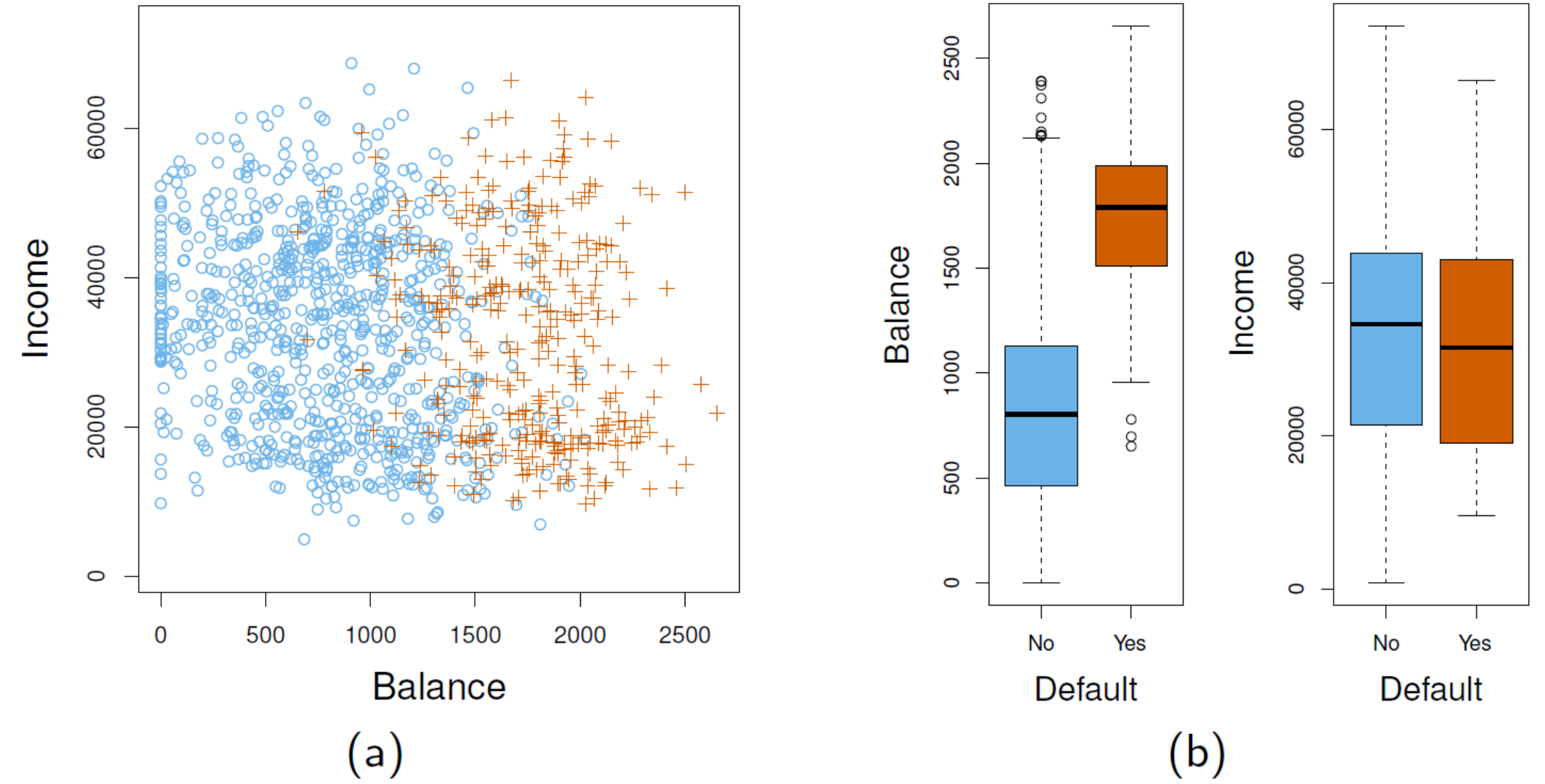
- (a): individual who defaulted on credit card payments are shown in orange, and those who did not are shown in blue
- (b): boxplots of balance/income as a function of default status
P[default=yes∣balance]: probability of default given balance
- can be estimated / predicted by regression analysis
- logistic regression: more appropriate than linear regression
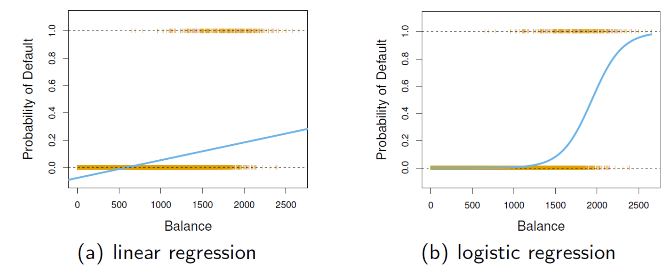
- estimated probability of default:
- (a): some probabilities are negative
- (b): all probabilities lie between 0 and 1
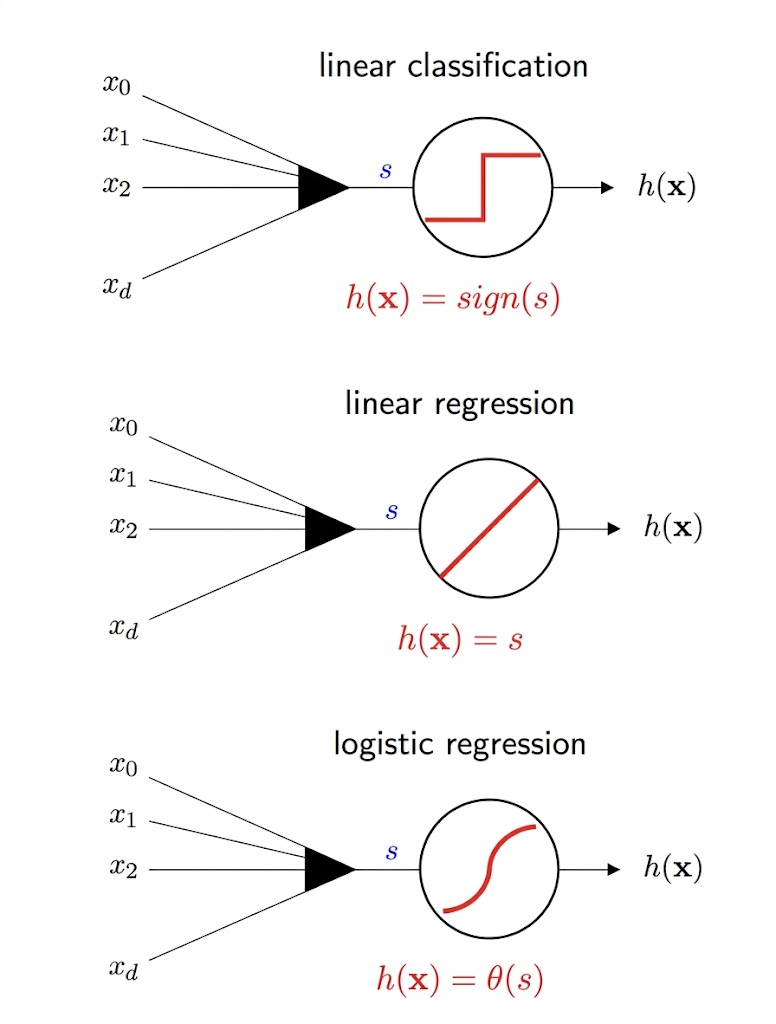
3. Logistic Regression Model
Linear Classification
- hard threshold on signal s=wTx
- h(x)=sign(wTx)
Linear Regression
- no threshold
- h(x)=wTx
Logistic Regression Model
- needs something between these two
- smoothly restricts output to probability range [0, 1]
- h(x)=θ(wTx)
- θ so-called logistic function
- 출력값의 특성
- 출력값이 실수이면서도 0과 1 사이로 제한적인 범위
- 임계값의 적용 방식
- 신호가 작을 때는 부드럽게 변하고 클 때는 선형 분류의 임계값에 수렴하는 형태
- 확실성 vs. 불확실성
- 연속적인 확률값으로 모델이 얼마나 확신/불확실한지 표현
3.1 Logistic Function θ
Definition
- For −∞<s<∞:
- θ(s)=1+eses=1+e−s1
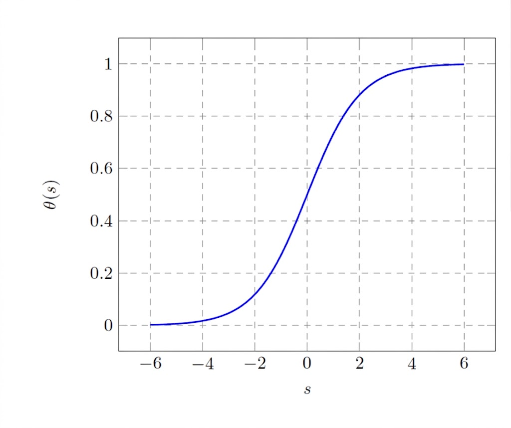
- output lies between 0 and 1
- can be interpreted as probability for binary events
- allow us to define an error measure that has analytical and computational advantages
- other names of logistic function θ
- soft threshold in contrast to the hard one in classification
- sigmoid its shape looks like flattened-out 's'
1−θ(s)=1−1+e−s1=1+e−se−s=θ(−s)
3.2 Linear Models
based on signal s=i=0∑dwixi
4. Example: Heart Attack
Prediction
- input x
- cholesterol level, age, weight, etc.,
- signal s=wTx
- risk score: 각 속성이 얼마나 중요한가/덜 중요한가?
Linear Classification
- h(x) returns ±1: heart attack (+1) or not (-1) for sure
Linear Regression
- h(x) returns risk score s itself
Logisitc Regression
- h(x) returns θ(s): probability of heart attack
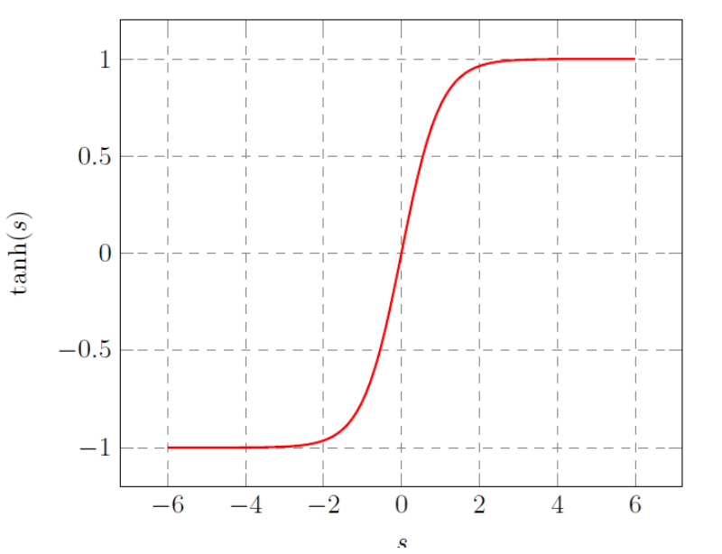
4.1 Another Popular Sigmod Function
Hyperbolic Tangent
- tanh(s)=es+e−ses−e−s
- tanh(s) converges to a hard threshold for large ∣s∣
- converges to no threshold for small ∣s∣
Linear, Logistic, Tanh, and Hard Threshold
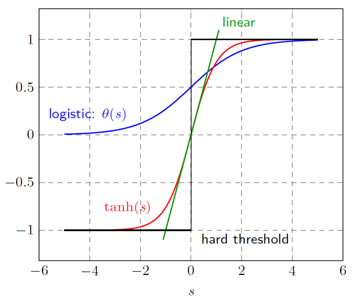
wTx= signal이고, 여기에 함수 f(s)=y 값을 만드는 과정을 activation이라고 부른다.
5. Learning Target and Error
5.1 Big Picture
- P[y=+1∣x]=f(x)∼h(x)=θ(wTx)
- P(y∣x)=h(x)[y=+1](1−h(x))[y=−1]=θ(ywTx)
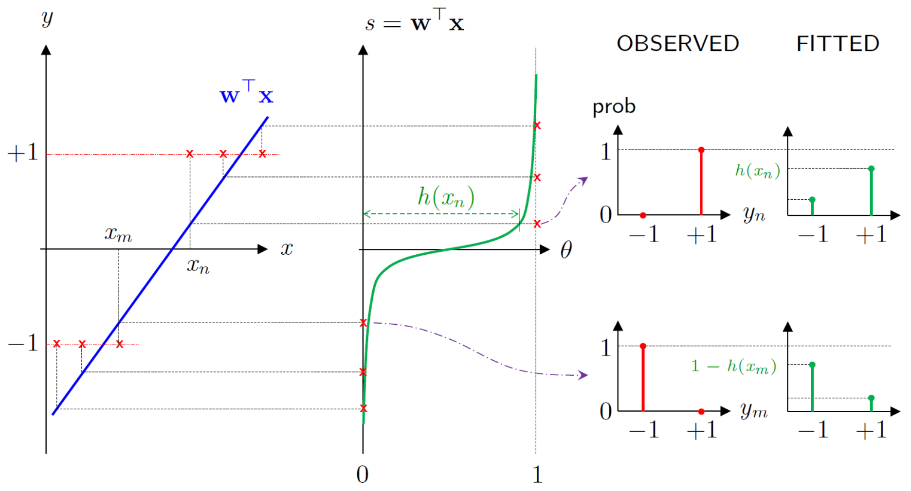
1. Linear Signal
- x→wTx
- 파란색 직선 wTx은 입력값 x를 받아 signal 혹은 risk score 계산
- wTx→θ(s)
- 녹색 곡선 θ은 직선으로 뻗어가는 신호 s를 받아 0과 1 사이의 매끄러운 확률값 h(x)로 변환
- 신호가 크고 양수일수록 확률은 1에 가까워지고, 크고 음수일수록 0에 가까워짐
Observed vs Fitted
- Observed
- 실제 데이터 yn는 +1, -1와 같이 이진 샘플로 주어짐
- 그래프에서는 확률이 0 또는 1인 극단적인 막대로 표시
- Fitted
- 모델 $h(x)가 내놓는 결과
- 0이나 1로 단정 짓지 않고, 0과 1 사이의 연속된 수치로 나타남
Fitted 막대들이 Observed 막대들과 최대한 비슷해지도록 만드는 것이 학습의 목표이다.
5.2 Target
Learning Target
- probability of event y=+1 given input x
- f(x)=P[y=+1∣x]
- e.g., probability of heart attack given patient characteristics
입력 x이 주어졌을 때, 결과 y가 +1이 될 확률을 구하는 함수 f(x)를 배우는 것이 학습이다.
Training Data
- do not give us the value of f explicitly
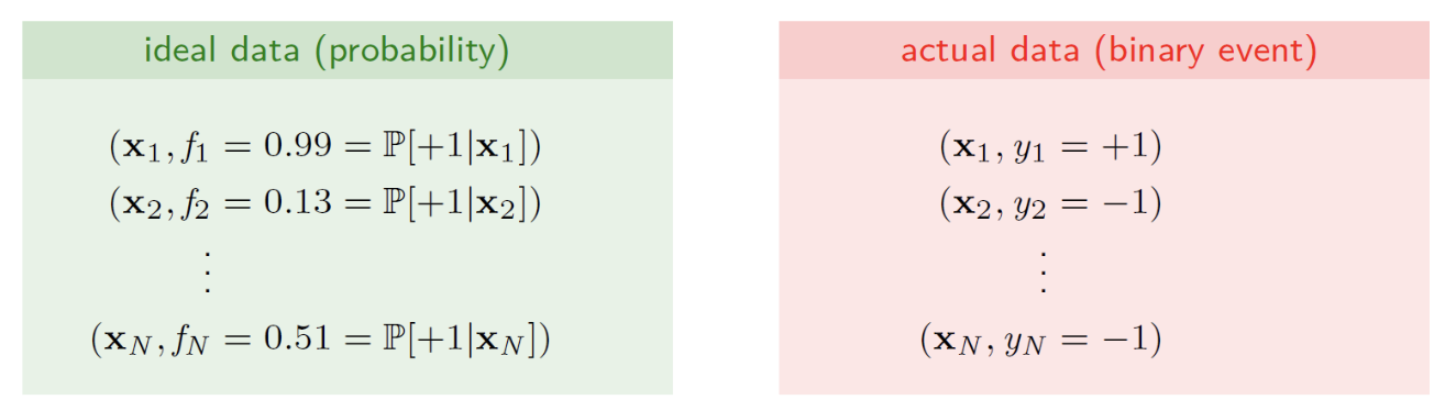
딱딱한 샘플들 yn만 보고, 부드러운 확률 분포 f(x)를 유추해내는 것이 학습의 핵심이다.
5.3 How to Measure Error?
- fitting data D means finding a good h
- h is good if
- h(xn)=1 whenever yn=+1
- h(xn)=0 whenever yn=−1
Simple
- not very convenient (hard to minimize)
Ein(h)=N1n=1∑N(h(xn)−21(1+yn))2
Cross-Entropy
looks complicated and ugly, but
- based on intuitive probabilistic interpretation
- has nice property for gradient-based optimization
- although not easy as linear regression
- yn=+1일 때
- 출력이 클수록 좋음
- θ는 1에 수렴, 오차는 0에 수렴
yn=−1일 때는 반대로 보면 된다.
6. Defining Error Measure
6.1 Likelihood & Maximum Likelihood
Likelihood
- standard error measure in logistic regression: likelihood
- how likely is it to get output y from input x, if target distribution P(y∣x) was indeed captured by h(x)?
P(y∣x)={h(x)1−h(x)for y=+1for y=−1
=θ(ywTx)
- h(x)=θ(wTx) and 1−θ(s)=θ(−s)
- this simplicity in: reason for defining θ(s) as es/(1+es)
Maximum Likelihood
- assume (x1,y1),...(xN,yN) are independently generated
- probability of getting all yn's from corresponding x's
P(y1∣x1)P(y2∣x2)…P(yN∣xN)=∏n=1NP(yn∣xn)
- the method of maximum likelihood
- select the hypothesis h that maximizes this probability
모든 데이터의 확률을 높이는 것은 모두 올바르게 분류하도록 만드는 것을 의미한다.
- equivalently minimize a more convenient quantity
- −N1ln(⋅) is monotonically decreasing function
−N1ln(n=1∏NP(yn∣xn))=N1n=1∑NlnP(yn∣xn)1
- substituting with p(y∣x)=θ(ywTx), we would be minimizing (wrt w)
N1n=1∑Nlnθ(ynwTxn)1=N1n=1∑Nln{h(xn)11−h(xn)1for yn=+1for yn=−1 (3)
=N1n=1∑N{[yn=+1]lnh(xn)1+[yn=−1]ln1−h(xn)1} (4)
[]는 안의 조건이 맞으면 1, 틀리면 0을 곱한다.
- 정답이 yn=+1일 때
- 왼쪽 항만 살아남고 오른쪽 항은 0을 곱해 사라짐
- 정답이 yn=−1일 때
매 데이터 포인트마다 정답에 해당하는 오차 딱 하나마 선택해서 계산하는 switch 구조이다. 수학적 최적화를 위해 합쳐서 사용한다.
6.2 In-sample Error Ein
- the fact that we are minimizing quantity (3)
- allow us to treat it as an error measure
- substituting the functional form for θ(ynwTx) produces
- in-sample error measure for logistic regression
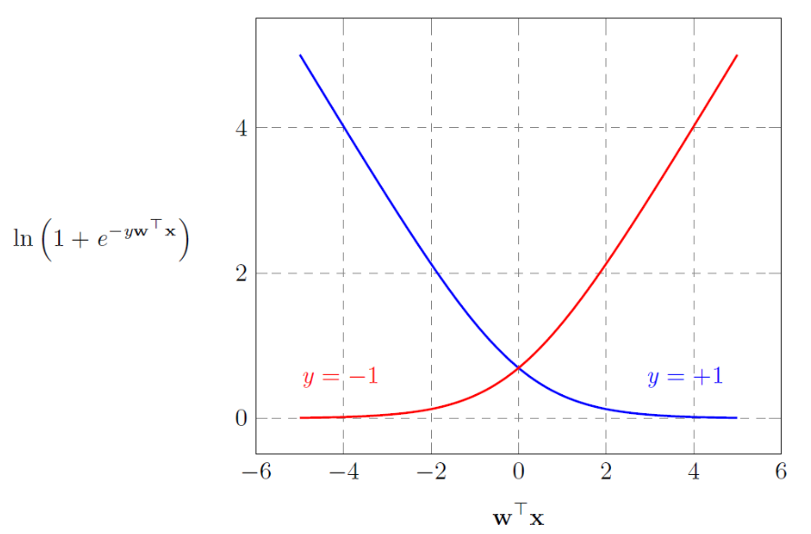
Ein(w)=N1n=1∑Nln(1+e−ynwTxn)
- implied pointwise error
- e(h(xn),yn)=ln(1+e−ynwTxn)
개별 오차들을 모두 더해서 데이터 개수로 나누면, 전체 평균 오차(Ein)가 완성된다.
6.3 Optimization
max∏n=1NP(yn∣xn)
⇔maxln(∏n=1NP(yn∣xn))
≡max∑n=1NlnP(yn∣xn)
⇔min−N1∑n=1NlnP(yn∣xn)
≡minN1∑n=1NlnP(yn∣xn)1
≡minN1∑n=1Nlnθ(ynwTxn)1 - h 대입
≡minN1∑n=1Nln(1+e−ynwTxn)
- small when yncTxn is large and positive
- which would imply that sign(wTx)=yn
- therefore, as out intuition expect
- the error measure encourages w to classify each xn correctly
- alternative derivation of Ein(w) is possible
- based on the notion of cross entropy
6.4 Cross-Entropy
- consider two pmfs p,1−p and q,1−q with binary outcomes
- cross entropy for these two pmfs: defined by
- plogq1+(1−p)log1−q1
- cross entropy measures the error for approximating
- observed(정답) pmf p,1−p by fitted(예측) pmf q,1−q
정답과 예측 사이의 거리를 계산하여 두 확률 분포가 얼마나 다른지 측정한다.
Recall
P(y∣x)={h(x)1−h(x)for y=+1for y=−1
위 식은 시그모이드 함수 θ의 대칭성을 이용하여 다음과 같이 간결하게 표현할 수 있다.
P(y∣x)=θ(ywTx)
또, 조건부 지수 표현을 사용하여 하나의 식으로 합쳐서 쓸 수 있다.
P(y∣x)=h(x)[yn=+1](1−h(x))[yn=−1]
- Likelihood of data
- 전체 데이터셋에 대한 우도 함수는 각 데이터 포인트 확률의 곱으로 나타낸다.
- n=1∏NP(yn∣xn)=n=1∏Nh(xn)[yn=+1](1−h(xn))[yn=−1]
Negative Log-Likelihood
우도 함수에 로그를 취하고 음수를 붙여 최소화 문제로 변환한다. N으로 나누어 평균적인 손실을 구한다.
NLL(w)∝−N1log{n=1∏NP(yn∣xn)}=−N1log{n=1∏Nh(xn)[yn=+1](1−h(xn))[yn=−1]}=N1n=1∑N{[yn=+1]logh(xn)1+[yn=−1]log1−h(xn)1}
위 식의 시그마 내부 항이 바로 Cross-entropy Loss이다.
Cross-entropy Loss = Log Loss
6.5 Bic Picture