5. Linear Model (2)

1. Regression

1.1 Definition

• a statical method to study relationship between $\mathbf{x}$ and y
  • $\mathbf{x}$: covariate / predictor variable / independent variable / feature
  • $y$: response / dependent variable
• training data $(\mathbf{x}_1, y_1)$, $(\mathbf{x}_2, y_2)$, ... , $(\mathbf{x}_N, y_N)$
  • noise is added to target $y_n = f(\mathbf{x}) + \epsilon$
  • $y \sim P(y|\mathbf{x})$ instead of $y = f(\mathbf{x})$

Goal

• find a model $g(\mathbf{x})$ that approximate $y_n$

1.2 Etymology

• re(back) + gression(going)
  • going back from data to formula
  • regression towards the mean
    • tail and short men tend to have sons with heights closer to mean

Simple Linear Regression

1.3 Linear Regression

• popular linear model for predicting a quantitative response
  • applies to real-valued target functions
  • long history in statistics, social and behavioral sciences
  • regression means $y$ is real-valued
    • inherited from statistics

Simple vs. Multiple

• $d = 1$: simple linear regression
  • one predictor
• $d \ge 2$: multiple linear regression
  • multiple predictor

Least Squares

• ordinary least squares
  • minimizes the sum of squared residuals
  • leads to a closed-form expression
• generalized least squares, iteratively reweighted least squares

Maximum Likelihood

• Ridge / Lasso regression
• least absolute deviation regression

Other Techniques

• Bayesian linear regression, principal component regression

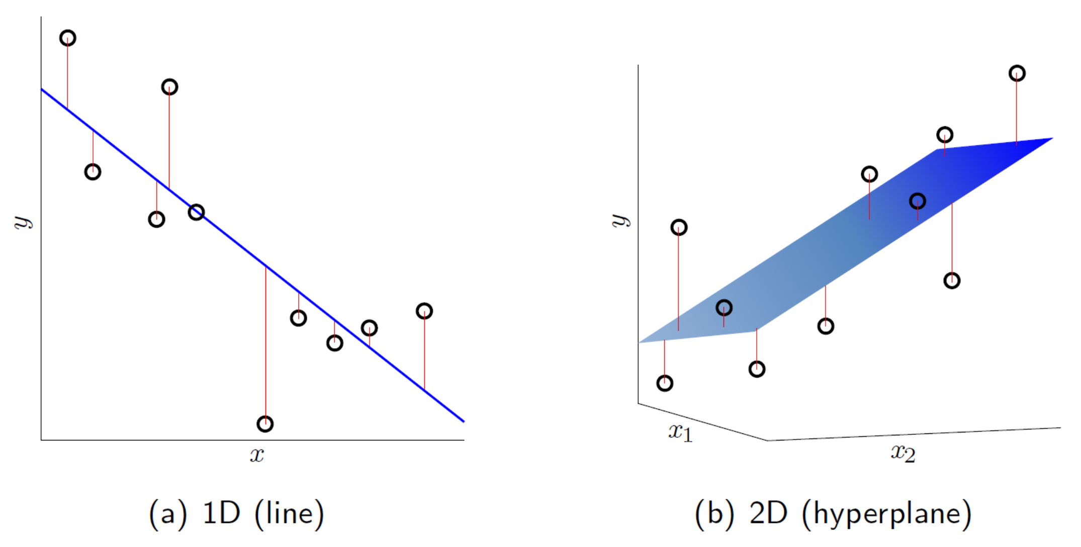
1.4 Linear Regression in 1D and 2D

• in OLS, sum of squared error is minimized
  • solution hypothesis (in blue) of linear regression algorithm in 1D and 2D

---

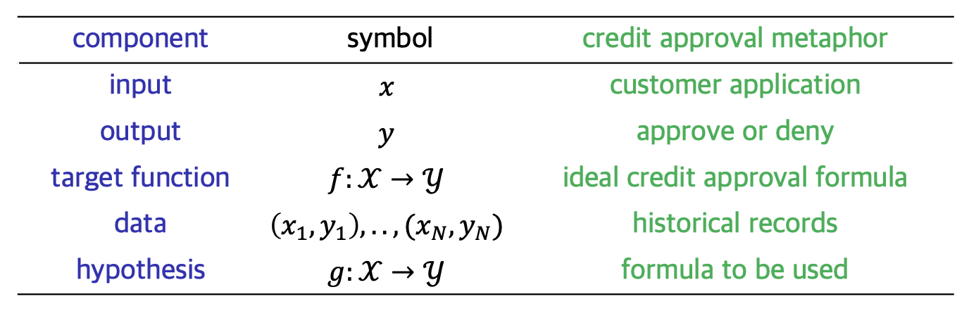
2. Credit Approval Revisited

2.1 Components of the Learning Problem

학습 문제의 핵심 요소를 추상화하기 위해 신용 승인 사례를 사용한다. 주요 구성 요소는 다음과 같다.

• $\mathbf{f}$: unknown target function
• $\mathbf{X}$: input space
• $\mathbf{Y}$: output space
• $N$: the number of input-output examples
  • i.e., training examples
• $D = {(x_1, y_1), ... , (x_N, y_N)}$: data set where $y_n = f(x_n)$

2.2 Regression Perspective

신용 승인 문제를 이진 분류가 아닌 회귀 관점에서 접근하면 다음과 같은 특징을 갖는다.

Quantitative Prediction

• consider credit approval as a regression problem
  • instead of making a binary decision
  • e.g., set a credit limit for each customer

Real-valued Target

• the bank uses historical records to build a data set $D$
  • $D:(\mathbf{x}_1, y_1), (\mathbf{x}_2, y_2),...,(\mathbf{x}_N, y_N)$
  • $\mathbf{x}_n$: customer information
  • $y_n$: credit limit
    • set by human experts; real number
    • $123,000 for Alicee and $57,000 for Bob

Automation

• the bank wants to automate this task (as it did with credit approval)
  • use learning to find a hypothesis $\mathbf{g}$

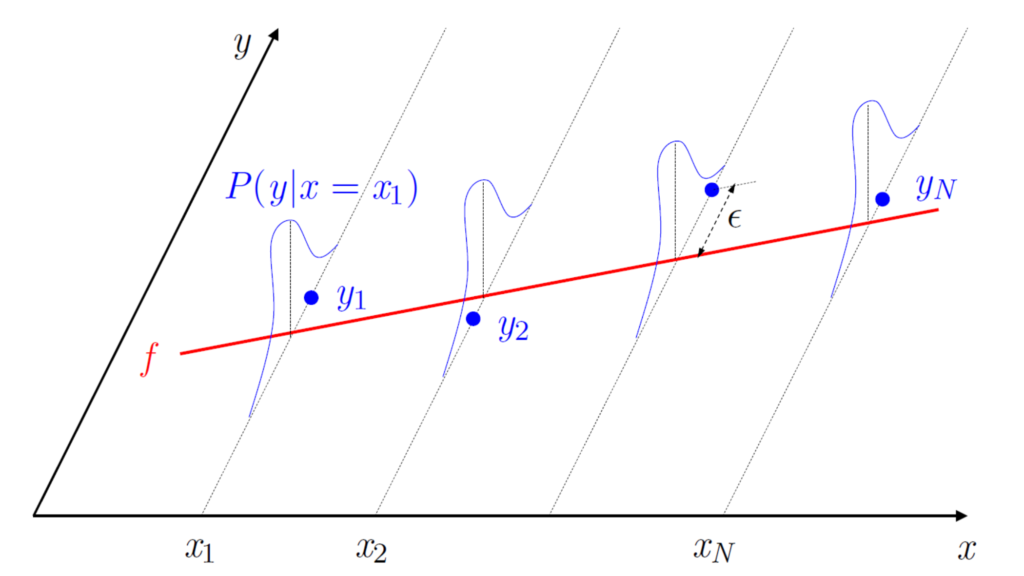
2.3 Target Distribution

현실적인 데이터 생성 과정에서는 완벽한 함수 $f$를 가정하기 어렵기 때문에 확률론적 관점을 도입한다.

Inconsistency of Experts

• each expert may not be perfectly consistent
• $\rightarrow$ out target will not be a deterministic function $y=f(x)$

Probabilistic Target

• regression label $y_n$ comes from some distribution $P(y|\mathbf{x})$ generating each $(\mathbf{x}_n, y_n)$
• instead of a deterministic function $f(\mathbf{x})$

Learning Goal

• we have a unknown distribution $P(\mathbf{x},y)$ generating each $(\mathbf{x}_n, y_n)$
• find a hypothesis $g$ that replicates how human experts determine credit limits
  • minimize the error between $g(\mathbf{x})$ and $y$ wrt that distribution $P$

학습 문제의 본질은 분류에서 회귀로 바뀌어도 변하지 않는다. 데이터를 통해 미지의 타겟을 근사하는 가설을 찾는다는 기계 학습의 기본 틀은 유지된다.

---

3. Linear Regression Algorithm

3.1 Error Measurement

• based on minimizing squared error between $h(\mathbf{x})$ and $y$
  • expected value is taken wrt joint probability distribution $P(\mathbf{x}, y)$

$E_{out}(h) = \mathbb{E} [(h(\mathbf{x}) - y)^2]$

Goal

• find a hypothesis $h$ that achieves a small $E_{out}(h)$

Issue

• $E_{out}$ cannot be computed
• since $P(\mathbf{x}, y)$ is unknown similar to what we did in classification

3.2 In-sample Error $E_{in}$

• resort to in-sample error instead:

Sum of Squared Residuals

$E_{in}(h) = \displaystyle \frac{1}{N} \sum^N_{n=1}(h(\mathbf{x}_n) - y_n)^2$

OLS는 잔차 제곱합을 최소화하는 기법이다. $E_{out}$은 $P(\mathcal{x}, y)$를 모르기 때문에 계산이 불가능하지만 $E_{in}$은 우리가 가진 데이터로 계산 가능하므로 $E_{out}$의 대리 지표로 사용한다.

Signal Representation

$h(\mathbf{x}) = \sum^d_{i=0} w_ix_i = \mathbf{w}^T\mathbf{x}$

• in linear regression, $h$ takes the form of
  • a linear combination of the components of $x$:
• $\mathbf{w}^T\mathbf{x}$: signal

항상 1의 값을 갖는 bias coordinate($x_0 = 1$)가 포함되어 있어 인덱스가 0부터 시작한다.