대기의 굴절률 변동은 random process이며, 이를 통과하는 광 경로 길이도 마찬가지로 무작위적입니다. 결과적으로 turbulence model들은 통계적 평균(structure function, 굴절률 변동의 power spectrum)을 준다. atmospheric phase screen을 만드는 문제는 random process를 개별 구현하여 생성하는 것이다. 그것은 컴퓨터가 생성한 난수들을 turbulence가 유도한 phase 변동과 같은 통계를 가진 sample point의 grid에서 2D 배열로 변환함으로써 phase screen이 만들어진다. 문헌에는 높은 계산 효율성, 높은 정확도 및 유연성을 갖춘 대기 위상 스크린을 생성하는 다양한 기법들이 많이 소개되어 있다.
보통 phase는 basis function의 가중치 합으로 표현한다. 보통 basis set은 Zernike polynomials와 Fourier series를 사용한다. 두 basis set은 장점과 단점이 있으며, 가장 흔한 방법은 McGlamery가 처음으로 도입한 FT 기반이다.
turbulence에 유도된 위상 가 Fourier 변환 가능한 함수라고 가정하면 Fourier 적분 표현으로
- phase의 공간 주파수 영역에서 표현
- power spectral density 의 random process 구현
- 2D 신호로 phase를 다룰려면, phase에서 총 power 는 power spectral density와 Parseval 정리(2가지 방법)으로 표현 가능하다.
유한 grid에서 phase screen 생성하기
유한 grid에서 phase를 생성하기 위해, optical phase 를 Fourier 급수로 표현하면
- 이산 x,y 공간 주파수
- Fourier 급수 계수
대기를 통한 phase 변동이 광경로를 통한 많은 random inhomogeneities 때문에, 우리는 가 가우시안 분포를 따른다는 것을 결정하기 위한 중심극한정리를 이용한다.
일반적으로, Fourier 계수 은 복소수이다.
실수, 허수부가 각각 평균 0이고 같은 분산을 가지고 cross-covariance가 0이을 가지도록 한다.
cross covariance
2개의 결합 정상 확률 과정 과 의 실제 cross covariance 시퀀스는 다음과 같이 평균이 제거된 시퀀스의 cross-correlation 이다.
- 는 두 정상 확률 과정의 평균값
결과적으로 그것은 평균이 0이고 분산이 인 복잡한 가우시안 분포를 따른다.
컴퓨팅 효율성을 위해 FFT를 사용하면, 주파수 샘플이 직교 grid에 선형적으로 spaced. 그리고 만약, grid size가 이면, 각각 주파수 spacing은 이면,
이제 문제는 Fourier 계수의 실현 값을 생성하는 것이다. 일반적인 random number는 평균 0, 분산 1인 가우시안 난수를 생성한다.
이것은 단순 변환을 요구한다.
를 이용하여 Gaussian 랜덤 변수를 평균 0, 1 분산으로 만들 수 있다. 이를 와 곱한 것은
위의 (Fourier 급수의 계수)를 랜덤 추출한다.
1. Pseudocode
FT를 이용하여 phase screen을 생성하는 코드
1. 의 값을 구한다.
2. frequency가 0인 성분의 phase을 0으로 설정한다. 이는 보통 신호의 평균값을 중심으로 phase 스펙트럼을 정규화
3. FS 계수를 랜덤 추출하여 생성한다.
FT를 사용하여 랜덤 추출로부터 phase screen을 합성한다.
- 실수와 허수 부분의 IFT는 2개의 uncorrelated phase screen을 생성하기 때문에
- 허수 부분은 지우고 실수 부분으로 부터 screen에 사용가능하다.
import numpy as np
import random

def ft_phase_screen(r0, N, delta, L0, l0):
    #### 1.Set up the Power Spectral Density ####
    delta_f = 1/(N*delta) # frequency grid spacing (1/m)
    fx_1d = np.arange(-N/2, N/2)*delta_f
    print(fx)

    fx, fy = np.meshgrid(fx_1d, fx_1d)
    f = np.sqrt(fx**2 + fy**2)
    theta = np.arctan2(fy, fx)

    fm = 5.92/(l0*2*np.pi)  # inner scale frequency [1/m]
    f0 = 1/L0               # outer scale frequency [1/m]

    # modified von Karman atmospheric phase PSD
    PSD_phi = 0.023*np.power(r0, -5/3) * np.exp(-(f/fm)**2) / np.power(f**2+f0**2, 11/6)
    # sets the zero-frequency component of the phase to 0
    PSD_phi[N/2, N/2] = 0
    ########

    # generatates a random draws of the FS coefficient
    c_n = (np.random.randint(N) + 1j*np.random.randint(n)) * np.sqrt(PSD_phi) * del_f

    # synthesize the phase screen from random draws using an FT
    ## real and imaginary parts of the IFT produce two uncorrelated phase screens.
    ### so use the scrren from real part and discard imaginary part
    phaze = np.real(np.ift2(cn,1))
1.1 한계점
위의 FFT 방법은 정확한 phase screen을 생성하지 못한다.
- , small-scale (high-frequency)
- , large-scale (low-frequency)
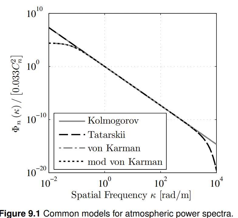
위 그래프에서 phase PSD(Power Spectral Density)가 대부분의 power를 mod von Karman(mvK) 모델이 낮은 공간주파수일 때 갖고 있다.
사실, tilt(기울기)와 같은 저차수 모드를 정확하게 표현하기 위해 공간 주파수 격자를 충분히 작게 샘플링하는 것이 종종 불가능하다는 점은 잘 문서화되어 있다.
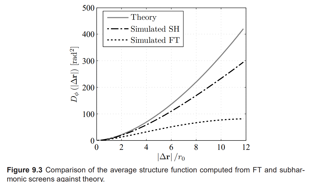
turbulence를 통한 예시 시뮬레이션을 위한 phase screen을 생성하고 확인할 때 아래 그림에서 이 차이가 분명해진다.(turbulence에서는 낮은 공간 주파수에 확연히 쏠림)
이 그림은 40 turbulent phase screen을 ft_phase_screen() 함수로 구현된 FT를 사용하여 생성한 것이다.
그리고, 각 screen의 structure 함수는 str_fcn2_ft 함수를 사용하여 계산된다. 그리고 결과가 평균화된다.
def str_fcn2_ft(phase, mask, delta):
    phase = phase * mask
    P = np.fft.fft2(phase)*delta
    S = np.fft.fft2(phase**2)*delta
    W = np.fft.fft2(mask) * delta
    delta_f = 1/(N*delta)
    w2 = np.fft.ifft2(W*np.conjugate(W)) * delta_f

    D = 2 * np.fft.ifft2(np.real( S * np.conjugate(W) - np.abs(P)**2)/delta_f / w2 * mask
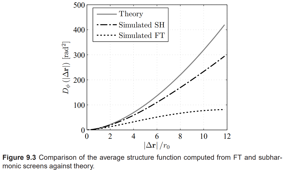
Average Structure 함수의 단면은 점선으로 표시된다. 분명히, screen의 통계는 실선 회색으로 표시된 Theory Structure 함수와 잘 맞지 않는다. 가장 일치하지 않는 부분은 큰 분리 거리()에서 나타나며, 이는 낮은 공간 주파수에 해당한다.
이 단점들을 완화할 여러가지 접근이 제안되었는데,
1. Zernike mode 통계를 사용한(Noll), Zernike 다항식(또는 선형 조합)의 랜덤 추출 방법
- Cochran
- Roddier
- Jakobssen
- 매우 낮은 주파수를 포함하기 위해, 공간 주파수 영역에서 불균일하게 sampling하는 FS 방법을 사용한 방법
- Welsh
- Eckert
- Goda
- 이 2가지 방법의 조합으로 subharmonics 가 제안되었는데, 저주파 Fourier 급수를 추가하여 FT screen을 보강한다.
- Herman and Strugala
- Lane et al
- Johansson and Gavel
- Sedmak
2. Lane et al의 subharmonic 방법
Frehlich가 이 screen을 사용하여 turbulent simulations으로 정확한 결과를 보여줬다.
low frequnecy screen phase는 아래처럼 다른 개 screen의 합이며, 에 대한 합은 이산 주파수에 걸쳐 있으며, index 의 각 값은 다른 grid에 해당한다.
2.1 Atmospheric phase-screen realization 생성
2.1.1 랜덤 추출로 atmospheric이 있는 phase screen 생성하기
주파수 영역에서의 신호 G를 다시 시간(또는 공간) 영역으로 변환하는 과정
G는 주파수 영역에서의 신호를 나타내는 2차원 배열modified von Karman
random coefficient multiply
fft.fftshift(G)
Shift zero-frequency component to the center of the spectrum.
- 주파수 영역의 데이터는 일반적으로 저주파 성분이 중앙에 위치하고 고주파 성분이 양쪽 끝에 위치합니다. 그러나
fft함수는 이와 다르게 데이터를 처리하기 때문에, 중앙에 저주파 성분이 오도록 데이터를 이동시키기 위해fftshift를 사용
fft.ifft2
- 2차원 역 푸리에 변환을 수행합니다. 주파수 영역의 신호 G를 다시 시간(또는 공간) 영역으로 변환
fft.ifftshift
- 다시 시간(또는 공간) 영역으로 변환된 데이터는 저주파 성분이 중앙에 위치. 이를 다시 원래의 순서로 되돌리기 위해
ifftshift를 사용곱셈 연산
- 결과에 (N delta_f) ** 2을 곱하는 이유는 푸리에 변환과 역 푸리에 변환은 스케일링 인자가 필요합니다. 2차원 데이터의 경우, (N delta_f) ** 2로 스케일링해 주어야 올바른 크기의 신호를 얻을 수 있습니다.
import numpy as np
import random

def ft_phase_screen(r0, N, delta, L0, l0):
    #### 1.Set up the Power Spectral Density ####
    delta_f = 1/(N*delta) # frequency grid spacing (1/m)
    fx_1d = np.arange(-N/2., N/2.)*delta_f

    fx, fy = np.meshgrid(fx_1d, fx_1d)

    f = np.sqrt(fx**2. + fy**2.)
    theta = np.arctan2(fy, fx)

    fm = 5.92/l0/(2*np.pi)  # inner scale frequency [1/m]
    f0 = 1/L0               # outer scale frequency [1/m]

    # modified von Karman atmospheric phase PSD
    PSD_phi = 0.023*np.power(r0, -5/3) * np.exp(-(f/fm)**2) / np.power((f**2+f0**2), 11/6)

    # sets the zero-frequency component of the phase to 0
    PSD_phi[int(N/2), int(N/2)] = 0
    ########

    # generatates a random draws of the FS coefficient
    cn = ( np.random.randn(N,N) + 1j*np.random.randn(N,N) ) * np.sqrt(PSD_phi) * delta_f

    # synthesize the phase screen from random draws using an FT
    ## real and imaginary parts of the IFT produce two uncorrelated phase screens.
    ### so use the scrren from real part and discard imaginary part
    g = np.fft.ifftshift(np.fft.ifft2(np.fft.fftshift(cn))) * (N * delta_f)**2
    phase = np.real(g)

    return phase
2.1.2 위의 FT method에 subharmonics를 보강한 코드
def ft_sh_phase_screen(r0, N, delta, L0, l0):
    """

    Creates a random phase screen with Von Karmen statistics with added
    sub-harmonics to augment tip-tilt modes.
    (Schmidt 2010)

        The phase screen is returned as a 2d array, with each element representing the phase change in [rad]
        this means that to obatain the physical phase distortion in [nm]
        it must be multiplied by (1/k)

    Args:
        r0 : screen in [m]
        N  : size of phase screen in [pixels]
        delta: size in [m] of each pixel
        L0: outer scale in [m]
        l0: inner scale in [m]

    Returns:
        representing phase screen in [radians]
    """

    D = N * delta

    # 1. High-frequency screen from FFT method
    phs_hi = ft_phase_screen(r0, N, delta, L0, l0)

    # 1.1 spatial grid [m]
    fx_1d = np.arange(-N/2, N/2)*delta
    x, y = np.meshgrid(fx_1d, fx_1d)

    # 2. Generating a low-frequency screen
    # 2.1 initialize low-frequency screen
    phs_lo = np.zeros(phs_hi.shape)

    # loop over frequency grids with spacing 1/(3^p*L)
    for p in range(1,4):
        # 3. Setup square root of the PSD
        # 3.1 frequnecy grid spacing = f_p = 1/(3**p*L)
        delta_f = 1/(3**p*D) # frequency grid spacing [1/m]
        fx_1d = np.array([-1,0,1]) * delta_f
        fx, fy = np.meshgrid(fx_1d, fx_1d)

        f = np.sqrt(fx**2+fy**2)
        theta = np.arctan2(fy,fx)

        fm = 5.92/l0/(2*np.pi)  # inner scale frequency [1/m]
        f0 = 1/L0  # outer scale frequency [1/m]

        # modified von Karman atmospheric phase PSD
        ##  fm = inner scale, f0 = outer scale
        PSD_phi = 0.023 * np.power(r0, -5/3) * np.exp(-(f/fm)**2) / np.power((f**2+f0**2), 11/6)
        PSD_phi[1,1] = 0

        # 3. Random draws of Fourier coefficient are generated
        # 3.1 random draws of Fourier coefficients
        cn = ( np.random.randn(3,3) + 1j*np.random.randn(3,3)) * np.sqrt(PSD_phi) * delta_f


        # 4. Sum over the n, m
        # 4.1 3 x 3 grid of frequencies for each p
        SH = np.zeros((N, N), dtype='complex')

        for n in range(0,3):
            for m in range(0,3):
                SH = SH + cn[n][m] * np.exp(1j*2*np.pi*(fx[n][m]*x+fy[n][m]*y))

        # 5. Sum over the N_p=3 different grids
        # accumulate subharmoics
        phs_lo = phs_lo + SH


    phs_lo = np.real(phs_lo) - np.mean(np.real(phs_lo))
    print(phs_hi)
    return phs_lo, phs_hi
2.1.3 최종 ft_sh_phase_screen 함수 실행
| parameter | value | --- |
|---|---|---|
| 2m | 정사각형 phase screen 한 변 길이 | |
| 0.1m | coherence 지름 | |
| 0.01m | inner scale | |
| 100m | outer scale |
import matplotlib.pyplot as plt
D = 2 # length of side of square phase screen [m]
r0 = 0.1 # coherence diameter [m]
N = 256 # number of grid points per side
L0 = 100 # outer scale [m]
l0 = 0.01 # inner scale [m]
delta = D/N # grid spacing [m]
# spatial grid
x = np.arange(-N/2, N/2) * delta
y = x
# generate a random draw of an atmospheric phase screen
phs_lo, phs_hi = ft_sh_phase_screen(r0, N, delta, L0 , l0)
phs = phs_lo + phs_hi
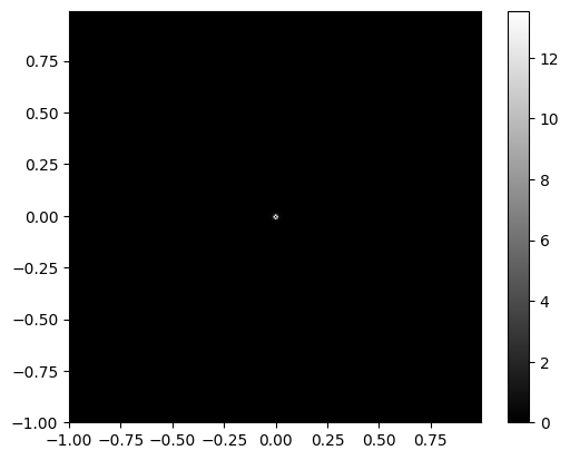
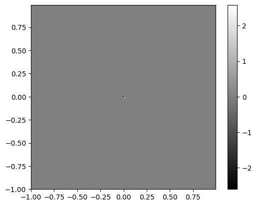
plt.title('Typical atmospheric phase screen created using SH')
plt.xlabel("$x [m]$")
plt.ylabel("$y [m]$")
plt.imshow(phs, cmap='gray', extent=(x.min(),x.max(), y.min(),y.max()))
plt.colorbar(label="$rad$")
plt.show()
몇몇 저자들이 subharmonic method의 능력을 조사했는데,
이 일을 처음으로 한 사람은 Herman and Strugala이고, 그들은 약간 subharmonic 방법의 다른 버전을 사용하는 동안, phase screen의 결과가 structure 함수가 이론이랑 잘 맞는 것을 보여준다.
그 subharmonic screen들로의 평균 Strehl ratio를 비교했다.
나중에, Lane et al이 특정 subharmonic 방법을 개발하고 이 screen 역시 이론적 structure 함수와 가까운것을 보여줬다.
곧이어, Johansson and Gavel은 Herman and Strugala와 Lane et al과의 방법을 비교했고, 자신의 subharmonic 방법이 더 이론에 structure 함수가 screen을 만드는 것을 보여줬다.
nonsquare subharmonic phase screen의 정확성을 조사하면서, Sedmak은 phase structure 함수와 aperture 평균 phase variance 간 좋은 일치를 보였다.
마침내, Frehlich가 subharmonic screen의 사용을 만드는 full wave-optics 시뮬레이션의 정확성을 연구했다.
- 그의 연구는 beam wave에 대해 irradiance 평균은 거의 FT screen과 subharmonic screen에 대해 정확하지만 subharmonic screen이 더 정확한 올바른 irradiance variance를 만든다.
- 평면파의 경우 두 method다 정확한 irradiance variances를 만들고, subharmonic method는 정확한 mutual coherence function을 만든다.