1. 연속형 변수

1. 기술통계량 : summarize_*( )

• 기술통계분석 : summarize(), summarize_at(), summarize_if(), summarize_all() 함수 이용

# tidyverse 라이브러리 구동
library('tidyverse’)
library('readxl’)
library('haven’)
library('magrittr’)
setwd(“______________”)
# 데이터 불러오기 및 사전처리 작업
data_131 = read_spss("data_TESS3_131.sav")
mydata = data_131 %>%
 mutate_if(
 is.double,
 funs(ifelse(. < 0,NA,.))
 )

# 한 개의 변수(연령 PPAGE)에 대한 기술통계치 구하기
mydata %>%
 summarize(mean(PPAGE,na.rm=T))
mydata %>%
 summarize(mean_ PPAGE =mean(PPAGE,na.rm=T))

#. A tibble: 1 × 1
mean(PPAGE, na.rm = T)

1 49.4
#. A tibble: 1 × 1
mean_PPAGE

1 49.4

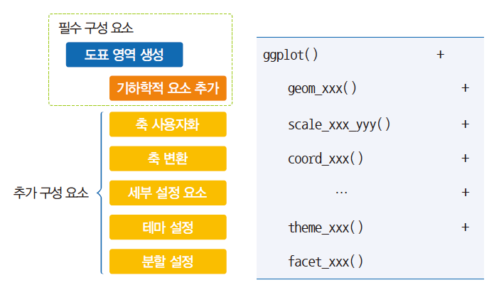
• ggplot2 패키지의 구성 요소
  • 기존에생성한도표영역위에 기하학적요소추가: + 연산자이용
  • 기하학적요소는함수명이geom_xxx() 형태
    

2. 기술통계량 : 시각화

• 평균과 95%의 신뢰구간 제시
• 박스플롯, 히스토그램, 빈도폴리곤 제시
  

# 박스플롯으로 시각화
g1=mydata %>%
 ggplot(aes(x="",y=PPAGE))+
 geom_boxplot()+
 coord_cartesian(ylim=c(15,90))+
 labs(x="",y="Age")+
 ggtitle("Box-Whisker plot")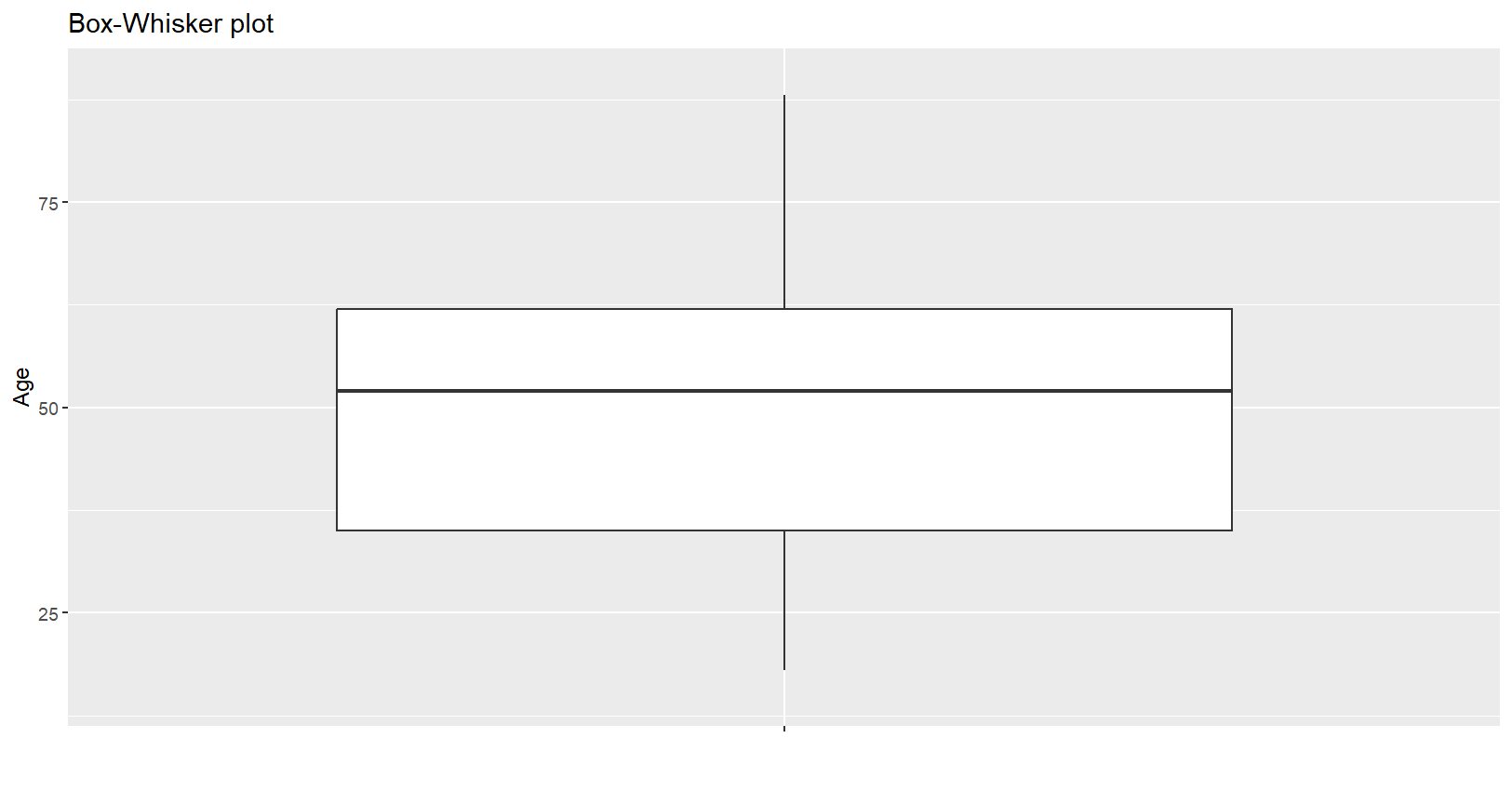

# 히스토그램으로 시각화
g2=mydata %>%
 ggplot(aes(x=PPAGE))+
 geom_histogram(bins=30)+
 coord_cartesian(xlim=c(15,90))+
 scale_x_continuous(breaks=c(15,10*(2:9)))+
 labs(x="Age",y="Frequency")+
 ggtitle("Histogram")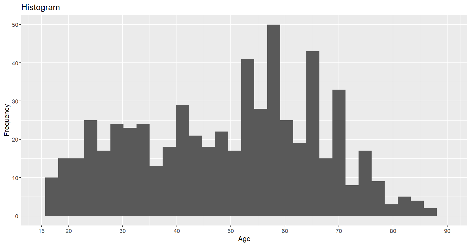

# 빈도 폴리곤
g3=mydata %>%
 ggplot(aes(x=PPAGE))+
 geom_freqpoly(bins=30)+
 coord_cartesian(xlim=c(15,90))+ 
 scale_x_continuous(breaks=c(15,10*(2:9)))+ 
 labs(x="Age",y="Frequency")+
 ggtitle("Frequency polygon")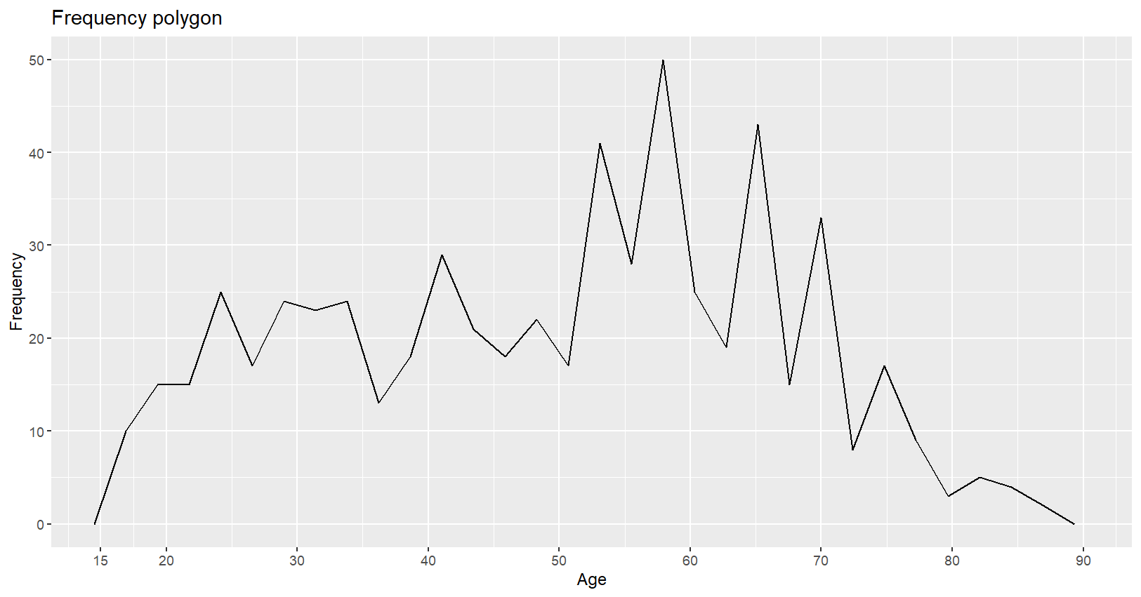

# 한번에 세 그래프 모두 그리기
gridExtra::grid.arrange(g1,g2,g3,nrow=1)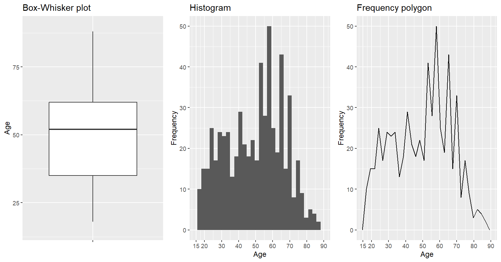

2. 기타 기술통계량 : sd, min, max

• 평균 외에 표준편차, 최소값, 최대값 등의 다른 통계량들도 summarize() 함수에서 활용 가능

# 변수: Q14
mydata %>%
 summarize(mean_Q14=mean(Q14,na.rm=T),
 sd_Q14=sd(Q14,na.rm=T),
 min_Q14=min(Q14,na.rm=T),
 max_Q14=max(Q14,na.rm=T))

3. summarize_*( )

• summarize_at( ) : 분석 대상이 되는 변수를 범위로 지정

# 여러 변수들(Q14:Q18)의 평균값 구하기
myresult = mydata %>%
 summarize_at(
 vars(Q14:Q18),
 funs(mean(.,na.rm=T))
 )
myresult

#. A tibble: 1 × 5
Q14 Q15 Q16 Q17 Q18

1 4.46 3.21 3.90 4.15 4.30

# 여러 변수들(Q14:Q18)의 평균값 → 시각화
myresult = myresult %>%
gather(key=Qs,value=Ms) 
# gather: 긴데이터로 형태 변환
# key: 데이터 변환시 데이터의 변수이름으로 변환되어 투입될 관측값을 갖
는 변수
# value: key로 지정된 변수에 해당되는 관측값
myresult %>%
ggplot(aes(x=Qs,y=Ms))+
geom_bar(stat="identity")+
coord_cartesian(ylim=c(2.5,5))+
labs(x="Statements",y="Average (5 = more important)")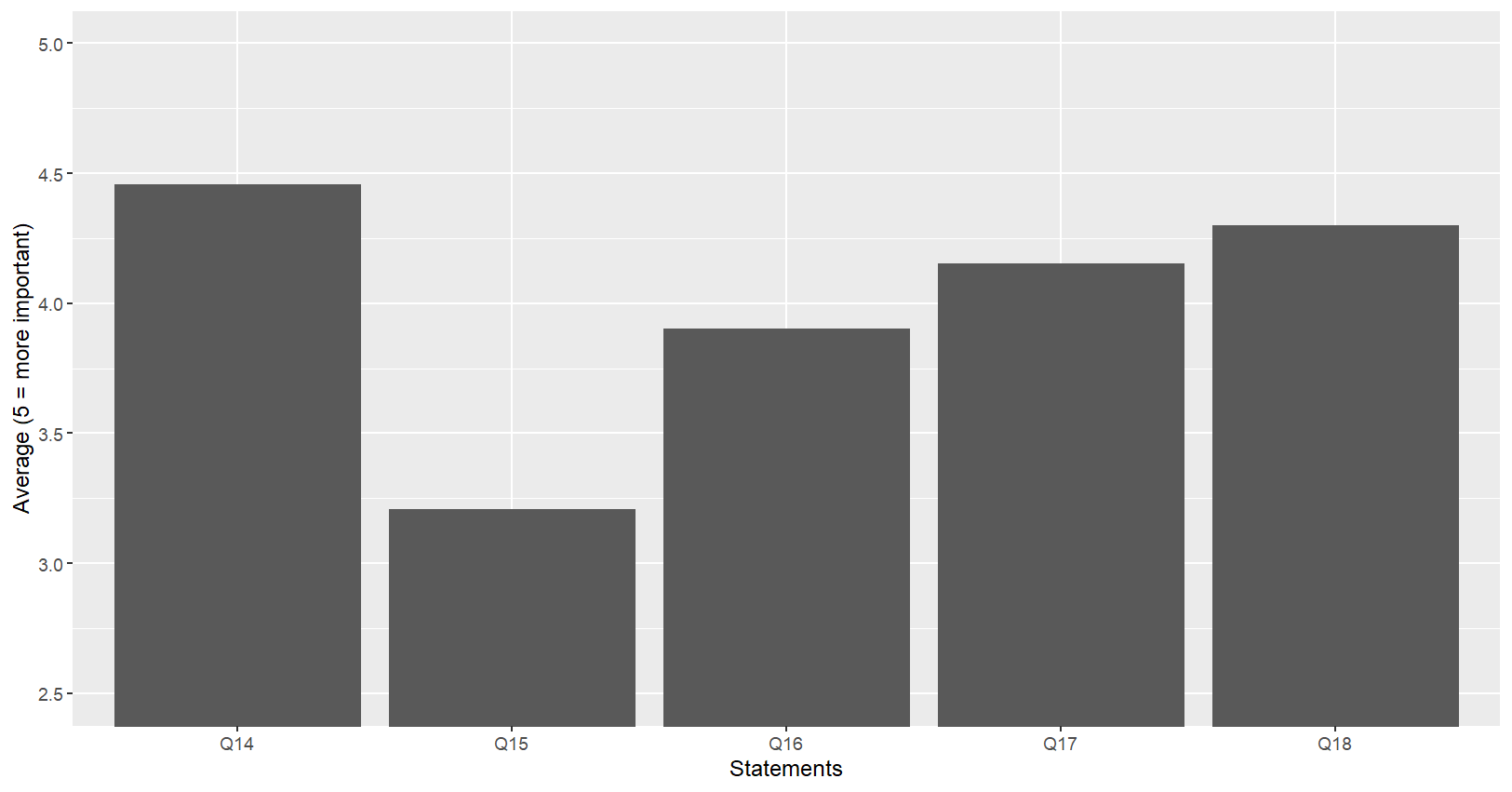

• fct_reorder(범주형변수, 기준변수, fun=함수, .desc=T/F)

# 보다 효과적인 시각화
myresult = myresult %>%
 mutate(
 mylbls=as.double(as.factor(Qs)),
 mylbls=labelled(mylbls, c(`Freedom of speech`=1,
 `Right to listen`=2,
 `Risk of violence`=3,
`Freedom to speak/hear`=4,
`Safety & security`=5)),
 mylbls=fct_reorder(as_factor(mylbls),Ms,"mean")
 ) 
myresult %>% ggplot(aes(x=mylbls,y=Ms))+
 geom_bar(stat="identity")+
 coord_flip(ylim=c(2.5,5))+
 labs(x="Statements",y="Average (5 = more important)")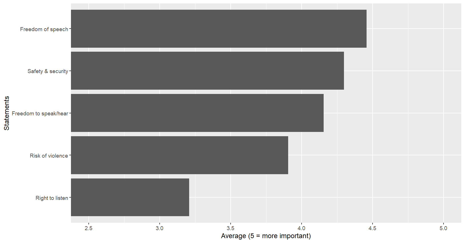

4. 연속형 변수 + 범주형 변수

• 응답자의 성별에 따라 해당 변수들의 평균값이 어떻게 다른가?

# 성별에 따라 Q14:Q18의 평균값들은 어떤 차이?
mydata = mydata %>%
 mutate(
 female=labelled(PPGENDER, c(male=1,female=2)), 
 female=as_factor(female)
 ) 
myresult = mydata %>%
 group_by(female) %>%
 summarize_at(
 vars(Q14:Q18),
 funs(mean(.,na.rm=T))
 )
myresult

#. A tibble: 2 × 6
female Q14 Q15 Q16 Q17 Q18

1 male 4.54 3.15 3.86 4.24 4.24
2 female 4.37 3.26 3.95 4.07 4.35

• 응답자의 성별에 따라 해당 변수들의 평균값이 어떻게 다른가?

# 시각화
myresult = myresult %>%
 gather(key=Qs,value=Ms,-female) %>%
 mutate(
 mylbls=as.double(as.factor(Qs)),
 mylbls=labelled(mylbls, c(`Freedom of speech`=1,
 `Right to listen`=2, 
`Risk of violence`=3, 
`Freedom to speak/hear`=4, 
`Safety & security`=5)), 
 mylbls=fct_reorder(as_factor(mylbls),Ms,"mean")
 )
myresult %>% ggplot(aes(x=mylbls, y=Ms, fill=female))+ #fill:비율
 geom_bar(stat=“identity”, position="dodge")+ #dodge:병치 
 coord_flip(ylim=c(2.5,5))+
 labs(x="Statements",y="Average (5 = more important)",fill="Gender")+
 theme(legend.position="top")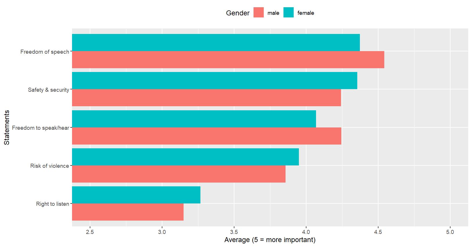

2. 상관분석

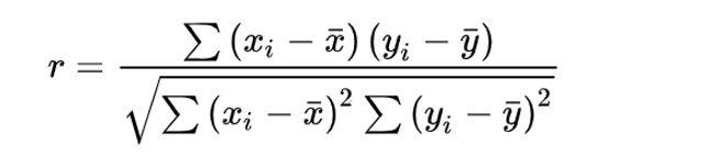
1. 피어슨 상관계수

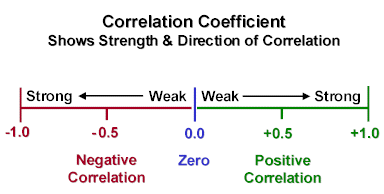
• 여러 다양한 상관계수들 중 하나, 가장 널리 사용되기 때문에 피어슨이라는 표현 없이 상관계수라고만 불리기도 함
• 두 개의 변수가 모두 연속형 변수일 경우, 두 변수의 선형관계(linear relationship)을 정량화 하는 수치
• 산점도(scatterplot)로 시각화
  
  
  
  

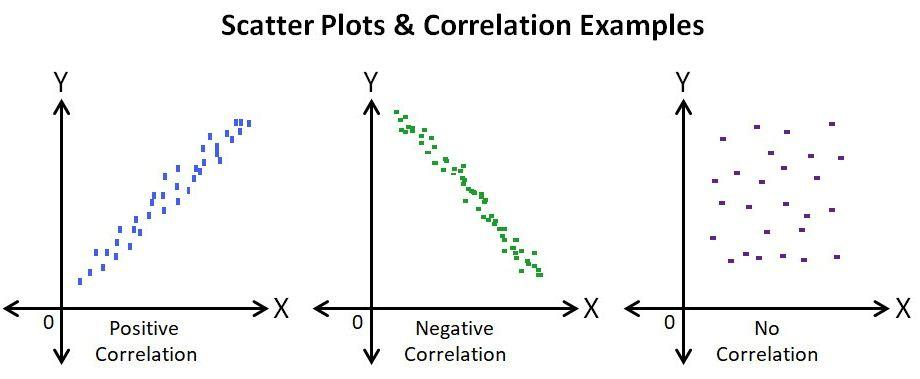
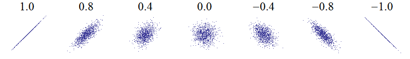
2. 산점도

• X축, Y축에 배치될 변수 모두 연속형 변수
• ggplot( ) + geom_point( ) 함수

# 전체도서관 수와 거주민 총수의 관계는?
mydata %>%
ggplot(aes(x=total,y=lib_tot))+
geom_point()+
labs(x="거주민 총수", y="도서관 총수")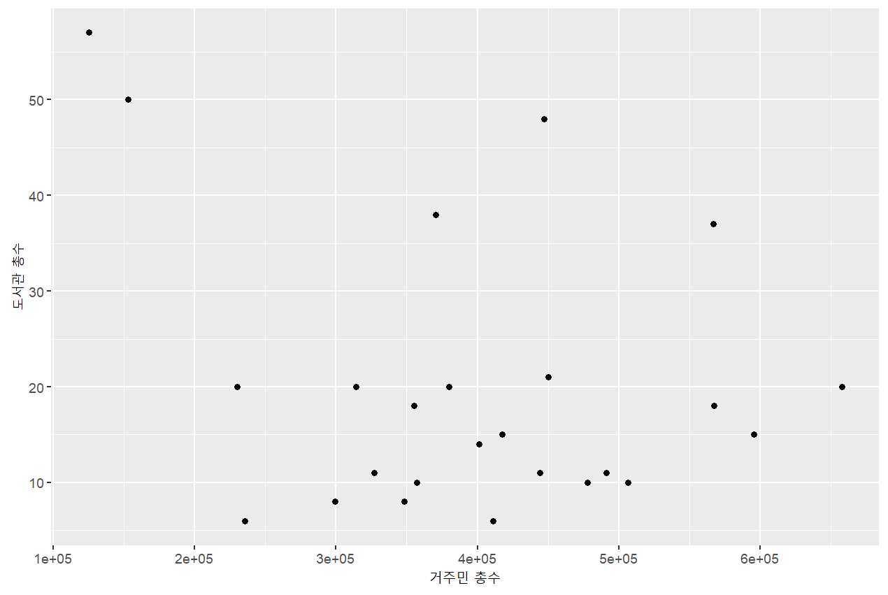 

# 전체도서관 수와 거주민 총수의 관계는? 
# X축 라벨이 1e+05 : 쉽게 해석 불가능 -> 라벨 교체
# X축 라벨을 10만명 단위로 나누고 표기를 “-만명＂으로 조정
mydata %>%
 ggplot(aes(x=(total/100000),y=lib_tot))+
geom_point()+
scale_x_continuous(breaks=0:7, labels=str_c(10*(0:7),"만명",sep=""))+
coord_cartesian(ylim=c(0,60), xlim=c(0.5,6.5))+
labs(x="거주민 총수",y="도서관 총수")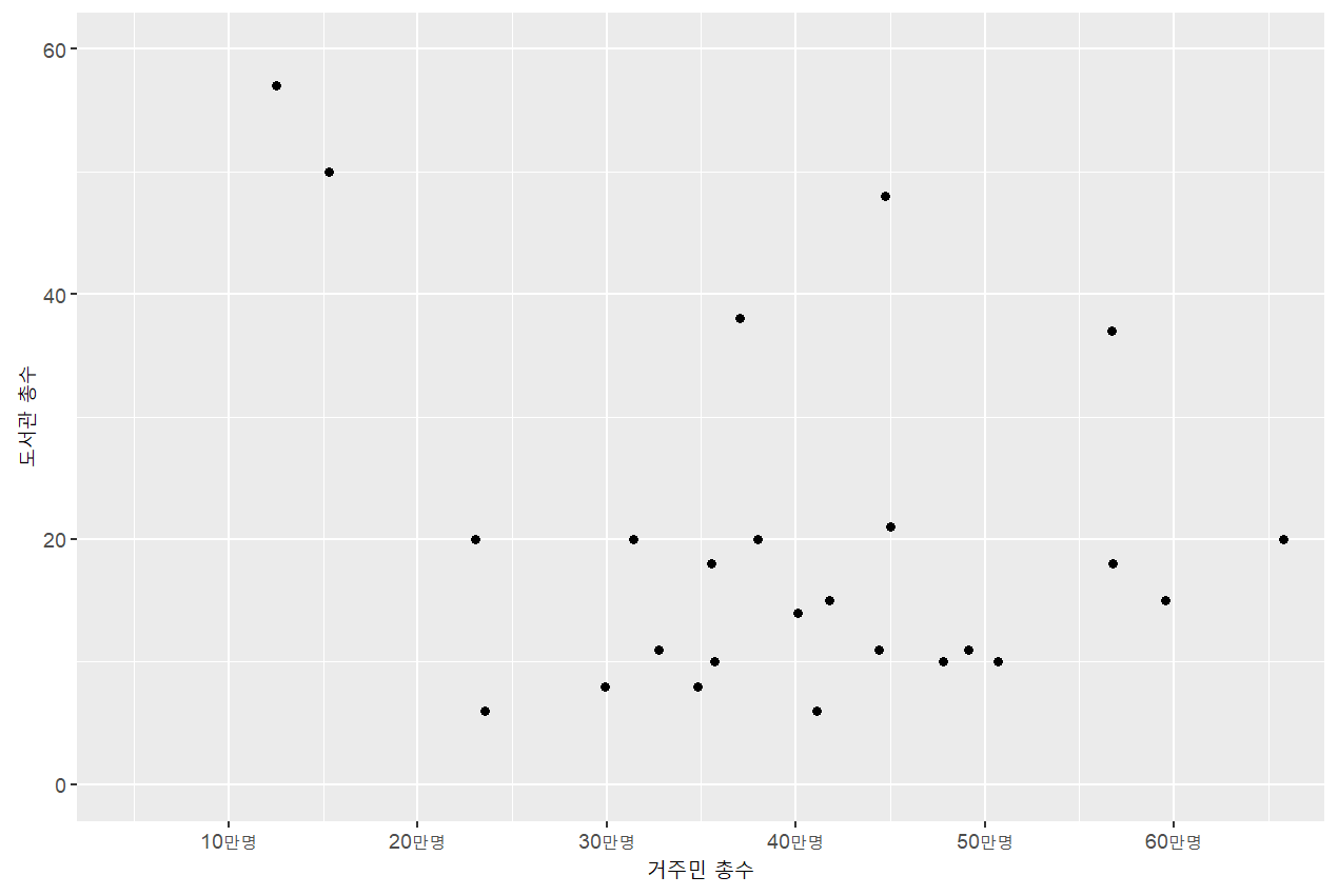

# 전체도서관 수와 거주민 총수의 관계는? 
# 각 점 대신 지역구의 이름을 표기
mydata = mydata %>%
mutate(
 district2=str_sub(district,1,2) # 첫 두 글자만 표기 (var, start, end)
 ) 
# aes 안에 label로 문자형 데이터 변수를 지정
# geom_text( ) 이용
mydata %>%
ggplot(aes(x=(total/100000),y=lib_tot, label=district2))+
geom_text()+
scale_x_continuous(breaks=0:7, labels=str_c(10*(0:7),"만명",sep=""))+
coord_cartesian(ylim=c(0,60),xlim=c(0.5,6.5))+
labs(x="거주민 총수",y="도서관 총수")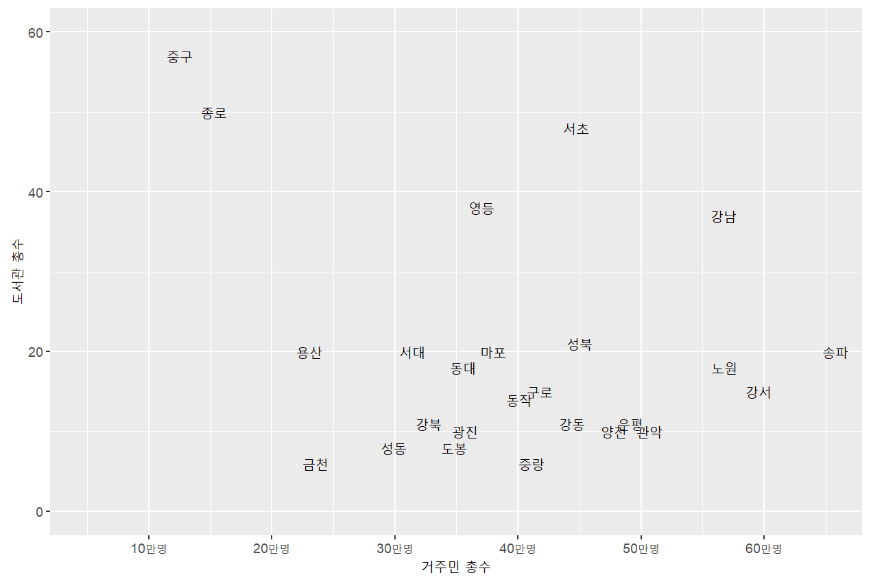

# 종로, 중구? 
# 전체도서관 = 국립 + 공공 + 대학 + 전문
# 도서관의 종류를 구분하자
# 도서관 유형별로 어떻게 다를까? 
mydata_long1 = mydata %>% 
 gather(key=lib_type, value=number, -(total:gen_100_),-year,-district,-district2)
mydata_long1 %>%
 filter(lib_type!="lib_tot") %>%
 ggplot(aes(x=(total/100000), y=number, label=district2))+
geom_text()+
scale_x_continuous(breaks=0:7,labels=str_c(10*(0:7),"만명",sep=""))+
coord_cartesian(xlim=c(0.5,6.5))+
labs(x="거주민 총수",y="도서관 총수")+
facet_wrap(~lib_type, ncol=2)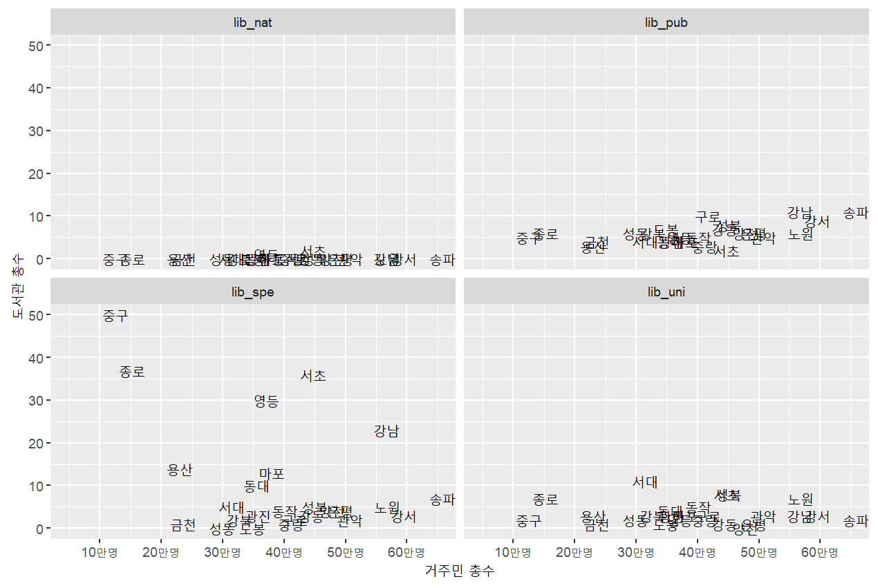

# 변수의 수준별 축의 범위가 다를 때 -> 표준화
# 표준화 방법
X
′ =
𝑋 − min(𝑋)
max 𝑋 − min(𝑋)
# 최소값=0, 최대값=1로 변환됨
# group_by( )를 이용해 도서관유형(lib_type) 변수 수준에 따라 도서관수(total)
를 표준화

# 도서관 유형별 도서관수를 0-1로 표준화
mydata_long1 %>%
 filter(lib_type!="lib_tot") %>%
 group_by(lib_type) %>%
 mutate(
 number2=(number-min(number))/(max(number)-min(number))
) %>%
ggplot(aes(x=(total/100000),y=number2,label=district2))+
 geom_text()+
 scale_x_continuous(breaks=0:7,labels=str_c(10*(0:7),"만명",sep=""))+
 coord_cartesian(xlim=c(0.5,6.5))+
 labs(x="거주민 총수",y="도서관 총수(0-1의 값으로 재조정)")+
 facet_wrap(~lib_type, ncol=2,
 labeller=as_labeller(c("lib_nat" = "국립도서관",
 "lib_pub" = "공공도서관", 
 "lib_spe" = "특별도서관",
 "lib_uni" = "대학도서관")))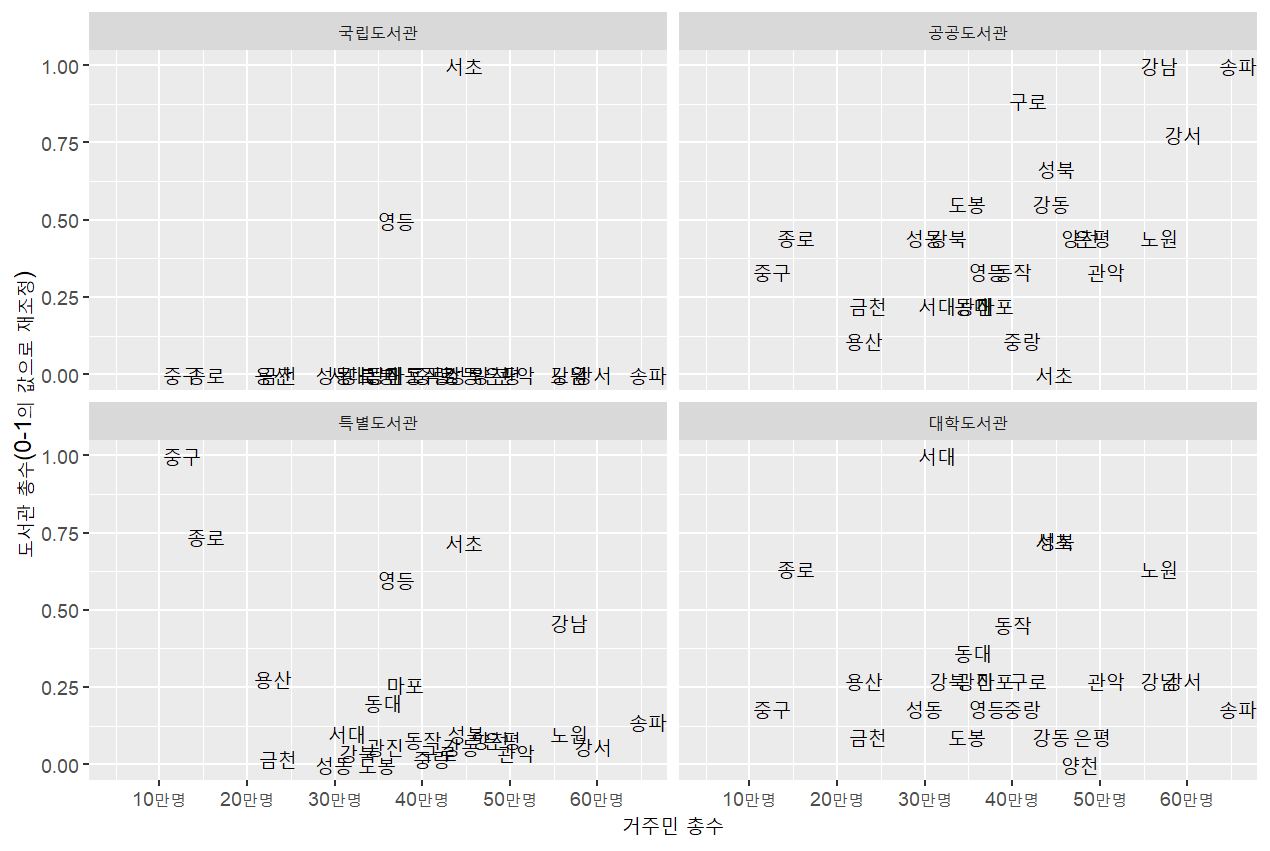

3. 피어슨 상관계수 r 계산

# 공공도서관수와 거주민수
(1) tidyverse library 이용: %>% 오퍼레이터 이용
mydata_long1 %>%
filter(lib_type==“lib_pub”) %>%
cor.test(~ total+number,data=.)
(2) R베이스 cor.test( ) 함수 이용: %$% 오퍼레이터 이용
mydata_long1 %>%
filter(lib_type=="lib_pub") %$%
cor.test(total, number)

# 공공도서관수와 거주민수
Pearson's product-moment correlation
data: total and number
t = 3.0373, df = 23, p-value = 0.005853
alternative hypothesis: true correlation is not equal to 0
95 percent confidence interval:
0.1774258 0.7678447
sample estimates:
 cor
0.5350465 

# 특별도서관수와 거주민수
mydata_long1 %>%
filter(lib_type=="lib_spe") %>%
cor.test(~ total+number,data=.)
Pearson's product-moment correlation
data: total and number
t = -2.0364, df = 23, p-value = 0.05338
alternative hypothesis: true correlation is not equal to 0
95 percent confidence interval:
-0.680829454 0.005072864
sample estimates:
 cor
-0.3908415 

# 대학도서관수와 거주민수
mydata_long1 %>%
filter(lib_type=="lib_uni") %>% 
 cor.test(~ total+number,data=.)
Pearson's product-moment correlation
data: total and number
t = -0.25929, df = 23, p-value = 0.7977
alternative hypothesis: true correlation is not equal to 0
95 percent confidence interval:
-0.4397365 0.3485808
sample estimates:
 cor
-0.05398585 

# 범주형 변수 수준별로 집단을 구분하여 상관계수 계산
# map( ) 함수 이용 : 모형추정 함수
# 데이터 입력 방식 주의
# 네 유형의 도서관 각각의 상관계수
mydata_long1 %>%
filter(lib_type!="lib_tot") %>%
split(.$lib_type) %>%
map(~ cor.test(~ total+number, data=.x))

# 네 유형의 도서관 각각의 상관계수
$lib_nat
Pearson's product-moment correlation
data: total and number
t = 0.25326, df = 23, p-value = 0.8023
alternative hypothesis: true correlation is not equal to 0
95 percent confidence interval:
-0.3496818 0.4387246
sample estimates:
 cor
0.0527356 
$lib_pub
Pearson's product-moment correlation
data: total and number
t = 3.0373, df = 23, p-value = 0.005853
alternative hypothesis: true correlation is not equal to 0
95 percent confidence interval:
0.1774258 0.7678447
sample estimates:
 cor
0.5350465 
$lib_spe
Pearson's product-moment correlation
data: total and number
t = -2.0364, df = 23, p-value = 0.05338
alternative hypothesis: true correlation is not equal to 0
95 percent confidence interval:
-0.680829454 0.005072864
sample estimates:
 cor
-0.3908415 
$lib_uni
Pearson's product-moment correlation
data: total and number
t = -0.25929, df = 23, p-value = 0.7977
alternative hypothesis: true correlation is not equal to 0
95 percent confidence interval:
-0.4397365 0.3485808
sample estimates:
 cor
-0.05398585 

# 정리된 결과 출력 : tidy( ) 함수 이용
# 네 유형의 도서관 각각의 상관계수
library(broom)
myresult = mydata_long1 %>%
filter(lib_type!="lib_tot") %>%
split(.$lib_type) %>%
map(~ cor.test(~ total+number,data=.x)) %>%
map_dfr(~ tidy(.))
myresult %>%
mutate(
 Pearson_r=format(round(estimate,3),3),
 p_value=format(round(p.value,3),3),
 what_i_want=str_c("r(",parameter,") = ",Pearson_r,", p = ",p_value) ) %>%
 select(what_i_want)

# 정리된 결과 출력 : tidy( ) 함수 이용
# 네 유형의 도서관 각각의 상관계수
# A tibble: 4 × 1
 what_i_want 
 <chr> 
1 r(23) = 0.053, p = 0.802 
2 r(23) = 0.535, p = 0.006 
3 r(23) = -0.391, p = 0.053
4 r(23) = -0.054, p = 0.798