
1. 추정
1. 추정방법
- 점추정 : 표본으로부터 추정량을 이용하여 모수를 추정하는 방법
- 표본추출에 따라 추정치가 달라지는 단점 존재
- 구간 추정 : 점추정을 중심에 두고 하한과 상한을 구하는 방법
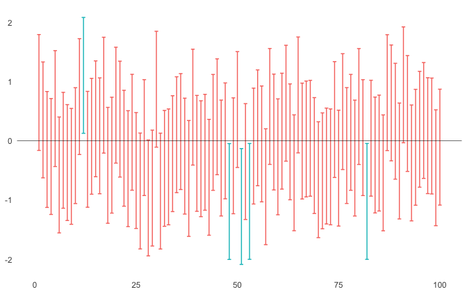
- 표준오차와 해당 추정치가 따르는 분포함수의 확률을 이용하여 신뢰구간을 구하는 과정
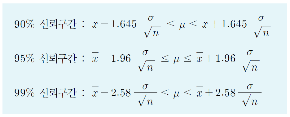
- 100(1-a)%신뢰구간:(1-a)로 표현하는 확률인 신뢰수준을 이용해 폭을 결정
2. 표본평균의 95% 신뢰구간 구하기
- 중심극한정리에 의해 모집단이 𝑋~𝑁(𝜇,𝜎^2)인 정규분포를 따를 때
- 표본평균은 X바~𝑁(𝜇,𝜎^2/𝑛)인 분포를 따르는 것을 확인
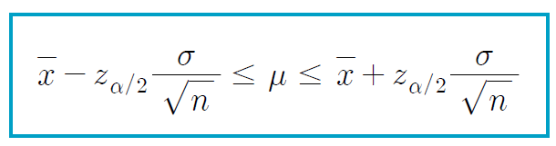
- 모분산이 알려진 정규모집단의 m에대한 100(1-a)% 신뢰구간
- 모집단이 표준정규분포이고, 표본의 크기가 4인 표본추출의 95% 신뢰구간을 구하는 과정
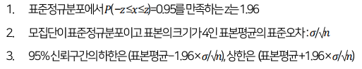
- 모집단이 표준정규분포이고, 표본의 크기가 n인 표본추출의 95% 신뢰구간을 구하는 과정
2. 가설검정
가설(Hypothesis)
모집단 상태에 대한 추측
- 주어진 사실 혹은 조사하고자 하는 사실이 어떠하다는 주장이나 추측
- 모수를 추정할 대, 모수가 어떠하다 (혹은 어떠할 것이다)는 조사자의 주장이나 추측
- 귀무가설, 대립가설
1-1. 귀무가설
- 일반적으로 믿어왔던 사실을 가설로 설정한 것
- 𝐻0으로 표기
- 모집단의 특성이 기존에 알려진 것과 "동일하다","차이가 없다"에 해당하는 가설
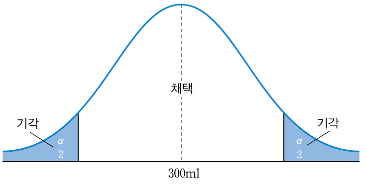
- ex, 스포츠 이온음료의 용량이 제품에 표시된 300ml가 맞는지에 대한 조사
- 귀무가설 : 스포츠 이온음료의 용량은 제품에 표기된 300ml가 맞다.
1-2. 대립가설
- 공공연하게 사실로 받아들여진 현상에 대립되는 가설
- H1으로 표기
- 귀무가설에 나타낸 모집단의 특성이 아니다, 기존에 알려진 것과
"다르다", "차이가 있다"에 해당하는 가설
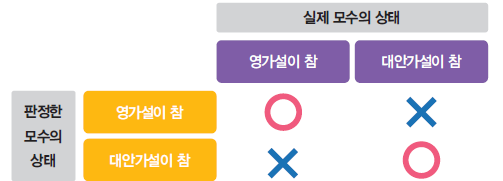
1-3. 유의수준
-
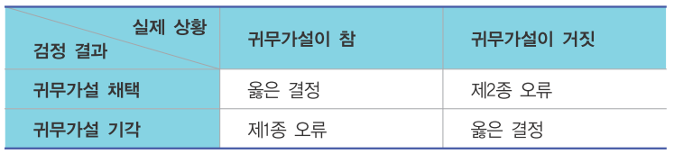
두가지 가설 중 하나를 선택하는 검정에서 발생할 수 있는 오류
-
제1종 오류 : 실제모수는 귀무가설이 참이지만, 대립가설을 채택하는 오류 . 알파로 표기
-
제2종 오류 : 실제모수는 대립가설이 참이지만, 귀무가설을 채택하는 오류 . 베타로 표기
검정력 : 1-베타 -
제1종 오류를 유의수준으로 사용
-
유의수준은 실험에서 설정함
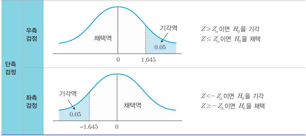
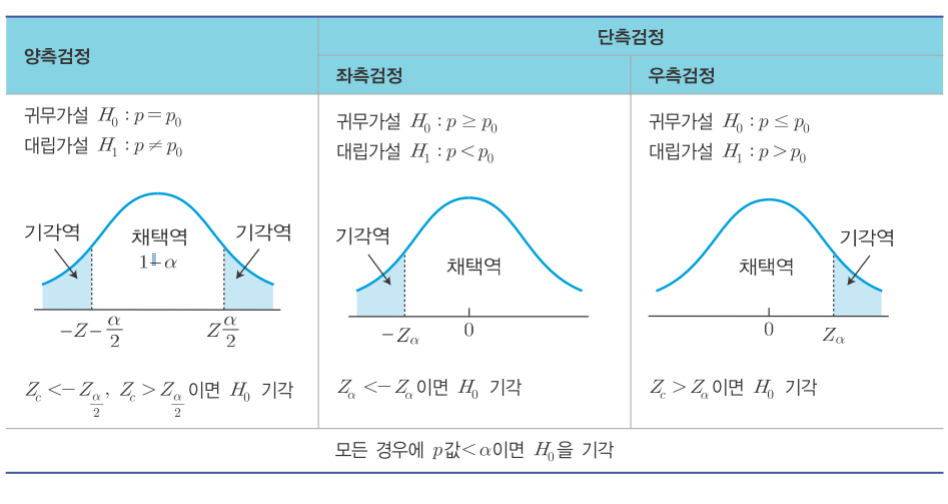
2. 양측검정과 단측검정
- 기각의 판단 기준은 양측검정과 단측검정으로 구분
- 조사 결과가 유의수준 알파에 포함되면 기각, 포함되지 않으면 채택
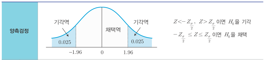
2-1. 양측검정(two-sided test)
- 조사하고자 하는 대립가설, 즉 '사실이 아니다'라는 것을 검정하여 귀무가설을 기각하고 대립가설을 채택하고자 하는것
- 귀무가설을 기각하고 대립가설을 채택할 수 있는 영역이 양쪽에 있는 경우
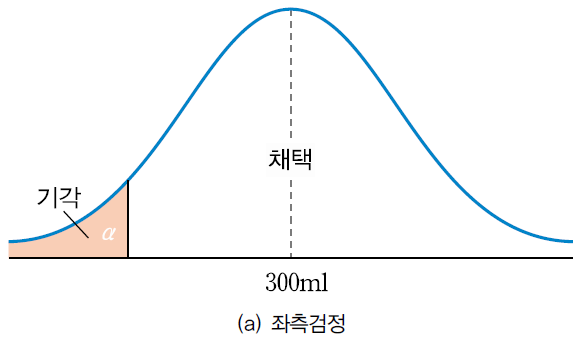
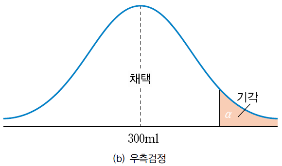
2-2. 단측검정(one-sided test)
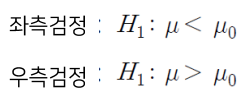
- 조사의 목적에 따라 대립가설을 스포츠 이온 음료의 용량이 300보다 적다 , 크다로 수립하여 한쪽만 보는 경우
- 귀무가설을 기각하고 대립가설을 채택할 수 있는 영역이 한 쪽에만 있는 경우
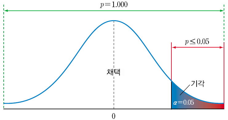
3. 유의확률(p-value)
- 유의수준에 따라 채택/기각을 결정한 지금까지의 방법은 신뢰범위에 포함되는지 그렇지 않는지만을 제시하므로 채택/기각에 대한 강도를 표현하기에는 충분하지않음
- 검정 통계량보다 더 극단적으로 값이 발생할 확률
- 검정통계량의 값 t에 대해 p-value=P(T>t)
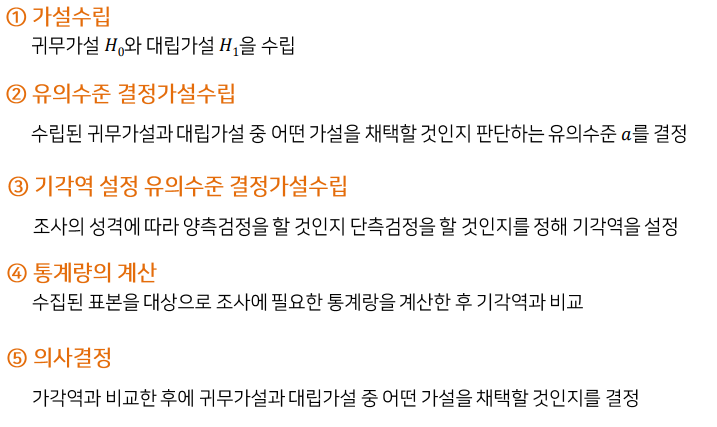
4. 가설검정의 절차
1. 모평균의 가설 검정
스포츠 이온음료의 용량이 제품에 표시된 3001교보다 모자라는 것 같아서 직접 조시를 해보고자 한다. 표본 300개를 대상으로 용량을 측정한 결과, 평균이 244.65로 확인되있다. 표준편차가 20일 때, 가설을 수립하고 유의수준 0.05에서의 좌측검정을 실시하라
-
귀무가설: 모평균이 특정 값과 동일
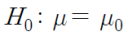
-
대립가설: (1) 양측검정의 경우, 모평균이 특정 값과 동일하지 않다
-
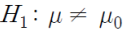
(2) 단측검정의 경우
-
t.test 이용
# MASS package에 포함되어 있는 cats data(Sex(성별), Bwt(몸무게), Hwt(심장무게)) 이용
library(MASS)
# H1: 몸무게의 평균이 2.6이 아니다.
t.test(cats$Bwt, mu=2.6)
One Sample t-test
data: cats$Bwt
t = 3.0565, df = 143, p-value = 0.002673
alternative hypothesis: true mean is not equal to 2.6
95 percent confidence interval:
2.643669 2.803553
sample estimates:
mean of x
2.723611
# H1: 몸무게의 평균이 2.7이 아니다.
t.test(cats$Bwt, mu=2.7)
One Sample t-test
data: cats$Bwt
t = 0.58382, df = 143, p-value = 0.5603
alternative hypothesis: true mean is not equal to 2.7
95 percent confidence interval:
2.643669 2.803553
sample estimates:
mean of x
2.723611# H1: 몸무게의 평균이 2.6보다 크다.
t.test(cats$Bwt, mu=2.6, alternative="greater")
One Sample t-test
data: cats$Bwt
t = 3.0565, df = 143, p-value = 0.001337
alternative hypothesis: true mean is greater than 2.6
95 percent confidence interval:
2.656656 Inf
sample estimates:
mean of x
2.723611# H1: 몸무게의 평균이 2.6보다 작다.
t.test(cats$Bwt, mu=2.6, alternative="less")
One Sample t-test
data: cats$Bwt
t = 3.0565, df = 143, p-value = 0.001337
alternative hypothesis: true mean is greater than 2.6
95 percent confidence interval:
2.656656 Inf
sample estimates:
mean of x
2.723611# H0: 몸무게의 평균은 2.6이다.
# 99% 신뢰구간
t.test(cats$Bwt, mu=2.6, conf.level=0.99)
One Sample t-test
data: cats$Bwt
t = 3.0565, df = 143, p-value = 0.002673
alternative hypothesis: true mean is not equal to 2.6
99 percent confidence interval:
2.618031 2.829191
sample estimates:
mean of x
2.723611# 성별에 따라 몸무게에 차이가 있는지 검정
# H0: 남녀간 평균 몸무게는 같다.
t.test(Bwt~Sex, data=cats)
Welch Two Sample t-test
data: Bwt by Sex
t = -8.7095, df = 136.84, p-value = 8.831e-15
alternative hypothesis: true difference in means is not equal to 0
95 percent confidence interval:
-0.6631268 -0.4177242
sample estimates:
mean in group F mean in group M
2.359574 2.900000# 성별에 따라 몸무게에 차이가 있는지 검정
# H0: 남녀간 평균 몸무게는 같다.
Bwt.f=cats$Bwt[cats$Sex=="F"]
Bwt.m=cats$Bwt[cats$Sex=="M"]
t.test(Bwt.f,Bwt.m)
Welch Two Sample t-test
data: Bwt by Sex
t = -8.7095, df = 136.84, p-value = 8.831e-15
alternative hypothesis: true difference in means is not equal to 0
95 percent confidence interval:
-0.6631268 -0.4177242
sample estimates:
mean in group F mean in group M
2.359574 2.900000▪ dataset: { 55,50,45,48,47,54,51,55,49,51}
▪ 귀무가설: 평균은 50이다.
▪ 대립가설: 평균은 50보다 크다
# default: 양쪽검정
x <- c(55,50,45,48,47,54,51,55,49,51)
dx<- x-50
t.test(dx)
One Sample t-test
data: dx
t = 0.464, df = 9, p-value = 0.6537
alternative hypothesis: true mean is not equal to 0
95 percent confidence interval:
-1.937584 2.937584
sample estimates:
mean of x
0.5- R에서는 기본적으로 양쪽검정을 수행
- 양쪽검정 결과 얻은 p-value를 2로 나누면 0.6537/2=0.32685
- p-value=0.32685 < 0.05 =𝛼
- 유의수준 5%에서 귀무가설 채택, 평균은 50이다.
# default: 양쪽검정
t.test(dx)
One Sample t-test
data: dx
t = 0.464, df = 9, p-value = 0.6537
alternative hypothesis: true mean is not equal to 0
95 percent confidence interval:
-1.937584 2.937584
sample estimates:
mean of x
0.5
# 한쪽 검정
x <- c(55,50,45,48,47,54,51,55,49,51)
dx<- x-50
t.test(dx,alternative = 'greater’ )
One Sample t-test
data: dx
t = 0.464, df = 9, p-value = 0.3268
alternative hypothesis: true mean is greater than 0
95 percent confidence interval:
-1.475268 Inf
sample estimates:
mean of x
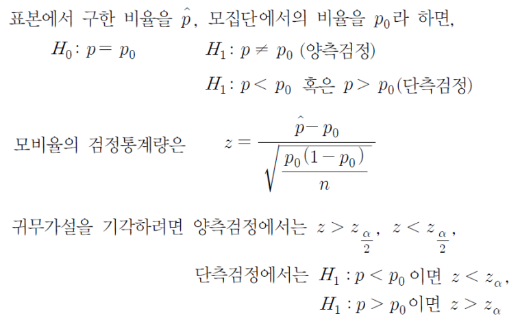
0.52. 모비율의 가설검정
s전자에서 AS 센터 서비스에 대한 불만이 민원으로 접수되이, 센터를 방문한 고객을대상으로 서비스 만족도를 조사하고자 한다. 방문한 고객의 80% 이상이 서비스에 만족한다면 서비스에 관한 재교육을 실시하지 않고, 그렇지 않다면 재교육을 실시할 예정이다.
무작위로 선택된 100명의 고객을 대상으로 만족도를 조사한 결과, 일명의 고객이 서비스에 만족한다고 했다. 이에 대해 유의수준 0.05에서 검정하라.
- 모집단에 대한 특성을 비율로 가늠하여 검정하는 것
- 조사 목적에서 목표로 하는 비율을 기준으로 제시하고, 조사 결과를 기준으
로 제시한 비율과 비교하여 높거나 혹은 낮으면 재택 또는 기각 - 예. 4번 타자가 되기 위해서는 3할(30%)을 넘어야 한다.
혹은 3할 3푼(33%)을 넘어야 한다는 등의 기준을 제시
# 표본크기 n=30, 앞면의 개수 x=18
# H1: 앞면이 나올 확률이 0.5가 아니다.
prop.test(x=18, n=30, p=0.5, alternative="greater")
1-sample proportions test with continuity correction
data: 18 out of 30, null probability 0.5
X-squared = 0.83333, df = 1, p-value = 0.1807
alternative hypothesis: true p is greater than 0.5
95 percent confidence interval:
0.4344744 1.0000000
sample estimates:
p
0.6
# H0: 4개 병원의 폐관련 질환 환자 수 대비 흡연자의 비율은 동일하다.
pa=c(86,93,136,82) # 4개 병원의 폐 관련 환자 수.
sm=c(83,90,129,70) # 폐 관련 환자 중 흡연자 수.# H0: 4개 병원의 폐관련 질환 환자 수 대비 흡연자의 비율은 동일하다.
pa=c(86,93,136,82) # 4개 병원의 폐 관련 환자 수.
sm=c(83,90,129,70) # 폐 관련 환자 중 흡연자 수.
prop.test(x=sm, n=pa)
4-sample test for equality of proportions without continuity correction
data: sm out of pa
X-squared = 12.6, df = 3, p-value = 0.005585
alternative hypothesis: two.sided
sample estimates:
prop 1 prop 2 prop 3 prop 4
0.9651163 0.9677419 0.9485294 0.8536585
# 4개 병원의 폐 관련 환자 수 대비 흡연자의 비율이 동일하다는 귀무
가설 기각500 명의 소비자를 대상으로 신규 출시하는 제품에 대한 선호도를 조사하였더니
이 중 86 명이 선호하는 것으로 나타났다. 이를 기초로 신규 출시하는 제품에 대한
선호율이 20%인지 유의수준 5%로 검정하라.
# 표본크기 n=500, x=86
# H0: 선호율은 20%이다.
prop.test(x=86, n=500, p=0.2, alternative="greater")
1-sample proportions test with continuity correction
data: 86 out of 500, null probability 0.2
X-squared = 2.2781, df = 1, p-value = 0.9344
alternative hypothesis: true p is greater than 0.2
95 percent confidence interval:
0.1450926 1.0000000
sample estimates:
 p
0.172
3. 여러개의 가설검정 동시에 수행
# 표본 4개
S1=c(89,90,92,66,44)
S2=c(56,66,77,90,44)
S3=c(67,80,91,99,34)
S4=c(45,34,56,82,34)
scores=data.frame(S1,S2,S3,S4)
scores
S1 S2 S3 S4
1 89 56 67 45
2 90 66 80 34
3 92 77 91 56
4 66 90 99 82
5 44 44 34 34
# 표본
4
개 summary
lapply
(scores,length
)
$S1
[1] 5
$S2
[1] 5
$S3
[1] 5
$S4
[1] 5
sapply
(scores,length
)
S1 S2 S3 S4
5 5 5 5tests=lapply(scores,t.test)
tests
$S1
One Sample t-test
data: X[[i]]
t = 8.1583, df = 4, p-value = 0.001229
alternative hypothesis: true mean is not equal to 0
95 percent confidence interval:
50.26735 102.13265
sample estimates:
mean of x
76.2
$S4
One Sample t-test
data: X[[i]]
t = 5.6182, df = 4, p-value = 0.004934
alternative hypothesis: true mean is not equal to 0
95 percent confidence interval:
25.39157 75.00843
sample estimates:
mean of x
50.2sapply(tests, function(t) t$conf.int) # tests=lapply(scores, t.test)
S1 S2 S3 S4
[1,] 50.26735 44.39538 42.55096 25.39157
[2,] 102.13265 88.80462 105.84904 75.00843