1. 등분산검정

1. 두 모집단 분산 동일성 검정

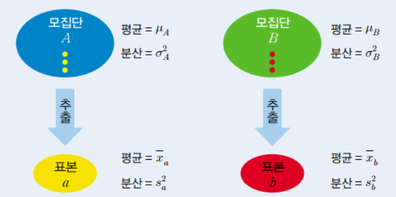
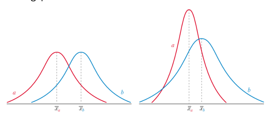
두 표본의 분포는 분산이 같은 경우와 분산이 같지 않은 경우를 나누어
생각

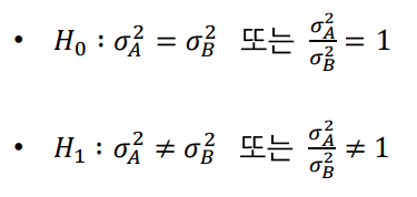
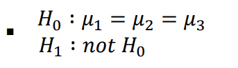
• 가설수립

  • 귀무가설: 두 집단의 모분산은 동일하다.
  • 대립가설:두집단의 모분산은동일하지 않다.

  

2.R등분산검정

# data 입력
sampleA <- c(2.1, 5.3, 1.4, 4.6, 0.9)
sampleB <- c(1.9, 0.5, 2.8, 3.1)
# 등분산 여부를 알기 위한 F검정
var.test(sampleA, sampleB)
F test to compare two variances
data: sampleA and sampleB
F = 2.8499, num df = 4, denom df = 3, p-value = 0.416
alternative hypothesis: true ratio of variances is not equal to 1
95 percent confidence interval:
 0.1887234 28.4398003
sample estimates:
ratio of variances
 2.849908 

# 등분산일 경우의 t-test
t.test(sampleA, sampleB, paired=F, var.equal=T)
Two Sample t-test
data: sampleA and sampleB
t = 0.69899, df = 7, p-value = 0.5071
alternative hypothesis: true difference in means is not equal to 0
95 percent confidence interval:
-1.870604 3.440604
sample estimates:
mean of x mean of y
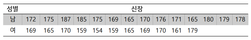
 2.860 2.075 

3.예제

다음 자료는 남학생과 여학생의 신장을 측정한 자료이다 이를 기초로 남녀간에 신장에 사이가 있는지 검정하라

# sleep data
?sleep
str(sleep)
head(sleep)
# 등분산검정
# t-test 검정

2. 분산분석(ANOVA)

1. 분산분석의 개념

• ANalysis Of VAriance : ANOVA
• 3개 이상의 집단에 대한 평균 사이를 검증하는 분석 방법
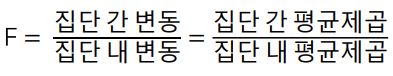
  • 특성에 대한 산포의 제곱합(분산)을 집단 내 분산, 집단 간 분산으로 분해한 후 그 비교를 통해 가설검정 수행.
• 집단 간의 분산이 크면 클수록,
  집단 내의 분산이 작으면 작을수록
• 집단 간의 평균 사이가 커짐
• 가설검정은 F분포를 이용
• 검정통계량F

• t검정에서는 직접적으로 두 집단에 대한 사이를 비교

• 3개 이상의 집단을 직접 비교하는 방법은 상당히 복잡
• 분산분석을 사용하는 것이 편리

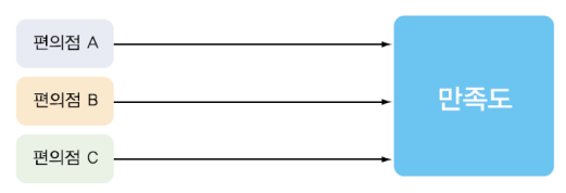
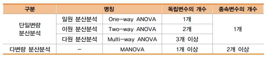
2-1. 일원 분산분석 (One-way ANOVA)

• 한 가지의 요인을 기준으로 집단 간의 사이를 조사하는 것
• 예. 편의점의 종류를 기준으로 고객의 만족도를 조사하는 경우
  

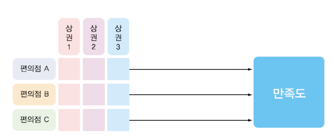
2-2. 이원 분산분석 (Two-way ANOVA)

• 두 가지 요인을 기준으로 집단 간의 사이를 조사하는 것
• 예. 편의점을종류와 위치를 기준으로나누고,
  편의점에 대한 고객의 만족도를 조사하는 경우
  

2-3. 다원 분산분석 (Multi-way ANOVA)

• 세 가지 이상의 요인을 기준으로 집단 간의 사이를 조사하는 것
• 예. 편의점의 종류와 상권, 본사 국가를 기준으로
  편의점에 대한 고객의 만족도를 조사하는 경우
  

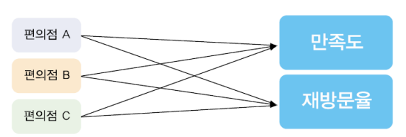
2-4. 다변량 분산분석 (Multi-variate ANOVA)

• 독립변수 1개 이상에 대해 종속변수 2개 이상으로 조사하는 것
• 예. 편의점의종류를독립변수로구성하고,
  종속변수로 고객의 만족도와 재방문율 2개로 구성하여 조사를 하는 경우
  

2. 분산분석의 구분

• 분산분석은 3개 이상의 집단에 대한 평균 차이를 알아보는 검정
• 독립변수와 종속변수의 개수에 따라 다음과 같이 구분됨

3. 분산분석의 가정

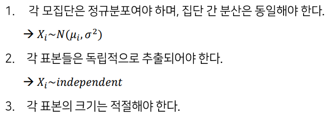
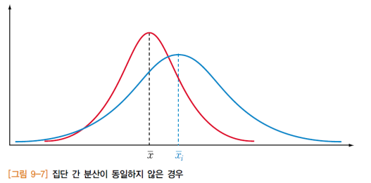
3-1. 각 모집단은 정규분포여야 하며, 집단 간 분산은 동일

• 모집단을 서로 비교하기 위해서는 각 모집단이 좌우대칭인 정규분포여야 하지만 집단 간의 평균은 서로 다를 수 있음
• 두 집단을 비교할 때 분산이 동일하지 않으면 집단 간의 평균 사이를 구별하기 쉽지 않음
• 분산분석은 집단이 3개 이상의 경우에 사용하는분석 방법이므로 분산이 다르면 계산이 어려워짐

3-2. 각 표본들은 독립적으로 추출

• 표본을 구성하는 과정에서 각각의 표본들은 모두 독립적으로 구성되어야 함
• 표본을 구성하는 과정에서 어느 집단이 다른 집단에 영향을 주지 않아야 함

3-3. 각 표본들의 크기는 적절

• 분석을 진행하기 위해서는 표본의 크기가 충분해아함
• 분산분석을 실시할 때 표본의 개수에 상관없이 분석을 진행할 수 있음

3. 일원분산분석

1. 일원 분산분석

• 하나의 독립변수를 3개 이상의 집단으로 나누어 각 집단의 분산을 고러
• 한 평균 사이가 통계적으로 유의한지 검정하는 방법
  두 집단의 평균 사이만 비교하는 독립표본 t검정의 확장
  • 귀무가설, 대립가설
  
• 서로 다른 집단쌍 수에 따라 독립표본 t검정을 여러 번 수행하지 않고 일
  원 분산분석을 수행
  • 반복해서 독립표본 t검정을 반복해서 수행하면 1종 오류(a)가 발생할 확률이
    증가하기 때문에 분산분석을 수행
• 분산분석 결과 귀무가설을 기각, 여러 집단 간 사이가 있는 것으로 나타남
  • 모든 집단 간에 차이가 있을 수도, 특정 집단 간에만 차이가 있을 수도
  • 어느 집단 간에 차이가 있는지 알고 싶으면 사후검정을 실시, 집단별로 통계적 비교를 수행

2. R함수

• aov(Y~x,data="dataset이름")
  Y : 정량적인수치
  x : 요인변수(factor)

• 분산분석에 앞서 정규성과 등분산성을 먼저 확인 (분산분석의 필요조건)

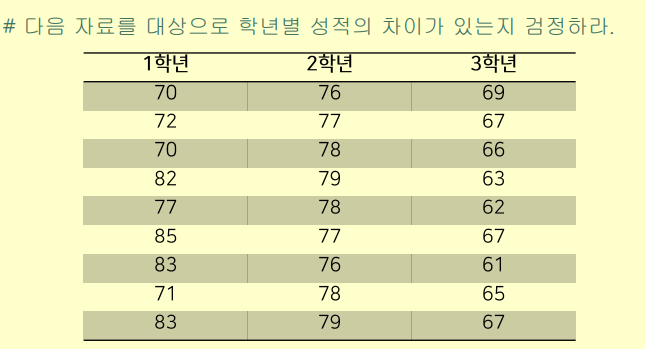
# data 입력
score01 <- c(80,82,80,82,77,85,83,81,83) #1학년 성적
score02 <- c(76,77,78,79,78,77,76,78,79) #2학년 성적
score03 <- c(65,67,66,63,62,67,61,65,64) #3학년 성적
scoreAll <- c(score01,score02,score03)
grade <- c(rep(1,9),rep(2,9),rep(3,9)) # 학년별로 각각 9 번 반복
# grade는 현재 수지 data의 요인으로 변경
grade <- factor(grade)
# 학년과 성적으로 table 생성
sampleData <- data.frame(scoreAll,grade)
sampleData

• 정규성 검정

# 정규성 검정을 위해 package 설치 및 불러오는 과정
install.packages(“nortest”)
library(nortest)
# Shapiro-Wilk normality test를 이용한 정규성 검정
tapply(scoreAll,grade,shapiro.test)

tapply(scoreAll,grade,shapiro.test)
$`1`
Shapiro-Wilk normality tes t
da ta: X[[i]]
W = 0.96156, p -value = 0.8145
$`2`
Shapiro-Wilk normality tes t
da ta: X[[i]]
W = 0.89939, p -value = 0.2485
$`3`
Shapiro-Wilk normality tes t
da ta: X[[i]]
W = 0.94253, p -value = 0.6088
# Shapiro-Wilk 정규성 검정 결과
1 학년의 p-value= 0.8145; 2 학년의 p-value=0.2485; 3학년의 p-value=0.6088
→ 유의수준 0.05수준에서 귀무가설을 채택
→ 학년별 성적은 정규성을 만족한다.

# 등분산 검정을 위해 library 설치 및 불러오는 과정
install.packages("car")
library(car)
# Levene's Test를 이용하여 등분산 검정
leveneTest(scoreAll ~ grade,data=sampleData)
Levene's Test for Homogeneity of Variance (center = median)
 Df F value Pr( >F)
group 2 1.12 0.3427
 24
# Levene 검정 결과: p-value=0.3427이므로 유의수준 0.05에서 귀무가설
을채택 → 학년별 분산은 서로 같다고 볼 수 있다.

• 학년별 평균 및 표준 편차

# 학년별 평균
aggregate(scoreAll~grade, sampleData, mean)
aggregate(list(meanScore = sampleData$scoreAll),
list(grade=sampleData$grade),mean)
grade meanScore
1 1 81.44444
2 2 77.55556
3 3 64.44444

# 학년별 표준편차
aggregate(scoreAll~grade, sampleData, sd)
aggregate(list(stdScore = sampleData$scoreAll),
list(grade=sampleData$grade),sd)
grade stdScore
1 1 2.297341
2 2 1.130388
3 3 2.127858

# 분산분석
result <- aov(scoreAll~grade, data= sampleData )
summary(result)
Df Sum Sq Mean Sq F value Pr( >F)
grade 2 1428.1 714.0 193.3 1.59e-15 ***
Residuals 24 88.7 3.7
---
Signif. codes : 0 ‘*** ’ 0.001 ‘**’ 0.01 ‘* ’ 0.05 ‘.’ 0.1 ‘ ’ 1

• 사후비교

# 사후비교
TukeyHSD(result)
Tukey multiple comparisons of means
95% family-wise confidence level
Fit: aov( formula = scoreAll ~ grade, da ta = sampleData)
$grade
 diff lwr upr p adj
2-1 -3.888889 -6.15164 -1.626138 0.0007102
3-1 -17.000000 -19.26275 -14.737249 0.0000000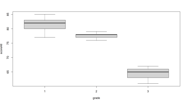
3-2 -13.111111 -15.37386 -10.848360 0.0000000

• 시각화
  #. boxplot
  boxplot(scoreAll~grade,data = sampleData)