딥러닝 - PyTorch: 프레임워크

1. 딥러닝의 기본 프레임워크

• Data Acquisition: 데이터 취득
• Preprocessing: 데이터 검증, 전처리 및 증강
• Modeling: 모델 설계
• Evaluation: 학습과정 추적, 후처리 및 모델 검증

---

2. PyTorch 기반 구현

2-1. Data Acquisition & Preprocessing

• 필요 데이터 로드 후 shape, dtype 확인
• 이미지 shape 표현 시 Tensorflow는 (batch, height, width, channel) 순서의 형태를 가지는 반면, PyTorch는 (batch, channel, height, width) 순서의 형태를 가짐
• PyTorch는 데이터셋 로딩 단계에서 전처리를 바로 적용할 수 있는 유연한 구조를 제공

from torchvision import datasets, transforms
from torch.utils.data import DataLoader

# 데이터 전처리 정의
transform = transforms.Compose([
	# 이미지를 Tensor로 변환
    transforms.ToTensor(), 
    # 픽셀값을 평균 0.5, 표준편차 0.5를 갖는 수로 정규화
    transforms.Normalize((0.5,), (0.5,))
])

# MNIST 데이터셋 로드
train_dataset = datasets.MNIST(
    root='./data',  # 데이터 저장 경로
    train=True,  # 학습 데이터 여부
    download=True,  # 필요 시 데이터 다운로드
    transform=transform  # 전처리 적용
)

test_dataset = datasets.MNIST(
    root='./data',
    train=False,
    download=True,
    transform=transform
)

# 데이터 로드
batch_size = 256

train_loader = DataLoader(
    dataset=train_dataset,
    batch_size=batch_size,
    shuffle=True  # 데이터 섞기
)

test_loader = DataLoader(
    dataset=test_dataset,
    batch_size=batch_size,
    shuffle=False
)

# 훈련 데이터 shape, dtype 확인
print("> Train data info")
print(f"Total length: {len(train_data)}")
print(f"Num of batches: {len(train_loader)}")
im, lbl = next(iter(train_loader))
print(f"Batch shape: IMG({im.shape}), LABEL({lbl.shape})")
# > Train data info
# Total length: 60000
# Num of batches: 235
# Batch shape: IMG(torch.Size([256, 1, 28, 28])), LABEL(torch.Size([32]))

# 테스트 데이터 shape, dtype 확인
print("> Test data info")
print(f"Total length: {len(test_data)}")
print(f"Num of batches: {len(test_loader)}")
im, lbl = next(iter(test_loader))
print(f"Batch shape: IMG({im.shape}), LABEL({lbl.shape})")
# > Test data info
# Total length: 10000
# Num of batches: 40
# Batch shape: IMG(torch.Size([256, 1, 28, 28])), LABEL(torch.Size([32]))

• 훈련 데이터 샘플 시각화

import matplotlib.pyplot as plt
im, lbl = next(iter(train_loader))
im_0 = torch.squeeze(im[0])
plt.figure(figsize=(2,2))
plt.imshow(im_0, cmap="grey")
plt.show()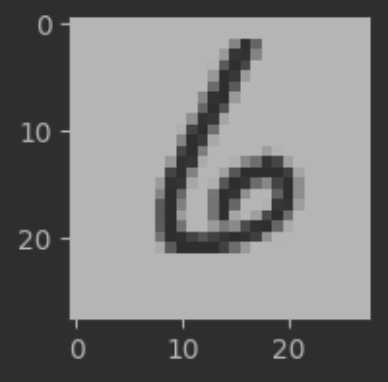

2-2. Modeling

• PyTorch에서는 통상적으로 레이어를 쌓을 때 torch.nn의 하위요소를 사용하고, 단순 활성화 함수를 사용할 때에는 torch.nn.functional의 하위 요소를 사용함
• 사용자 정의 모델을 설계할 때에는 torch.nn.Module을 상속받아 구성할 수 있음

import torch.nn as nn
import torch.nn.functional as F

class SimpleCNN(nn.Module):

	# 레이어(nn) 선언 부분
    def __init__(self):
        super(SimpleCNN, self).__init__()
        self.conv1 = nn.Conv2d(in_channels=1, out_channels=32, kernel_size=3, stride=1, padding=1)      
        self.conv2 = nn.Conv2d(in_channels=32, out_channels=64, kernel_size=3, stride=1, padding=1)      
        self.dropout = nn.Dropout(0.25)       
        # Flatten 후 연결 레이어 (64*7*7은 두번의 Conv, Max Pool 레이어를 거친 후의 형태)
        self.fc1 = nn.Linear(64*7*7, 128)     
        # 출력 레이어
        self.fc2 = nn.Linear(128, 10)
    
    # 레이어 간 연결 정의 부분
    def forward(self, x):
        x = self.conv1(x) # (batch, 32, 28, 28)
        x = F.relu(x)
        x = F.max_pool2d(x, 2, 2)  # (batch, 32, 14, 14)
        x = self.conv2(x)  # (batch, 64, 14, 14)
        x = F.relu(x)
        x = F.max_pool2d(x, 2, 2)  # (batch, 64, 7, 7)
        x = self.dropout(x)
        x = x.view(x.size(0), -1) # Flatten 처리 (batch, 64*7*7)
        x = self.fc1(x) # (batch, 128)
        x = F.relu(x)
        x = self.fc2(x) # (batch, 10)
        return F.log_softmax(x, dim=1)

• GPU 활성화 (AMD GPU 환경은 mps, NVIDIA GPU 환경은 cuda 사용)

device = torch.device("mps" if torch.backends.mps.is_available() else "cpu")
print(device) # mps

• 모델 생성

model = SimpleCNN().to(device) # GPU 사용 설정
print(model)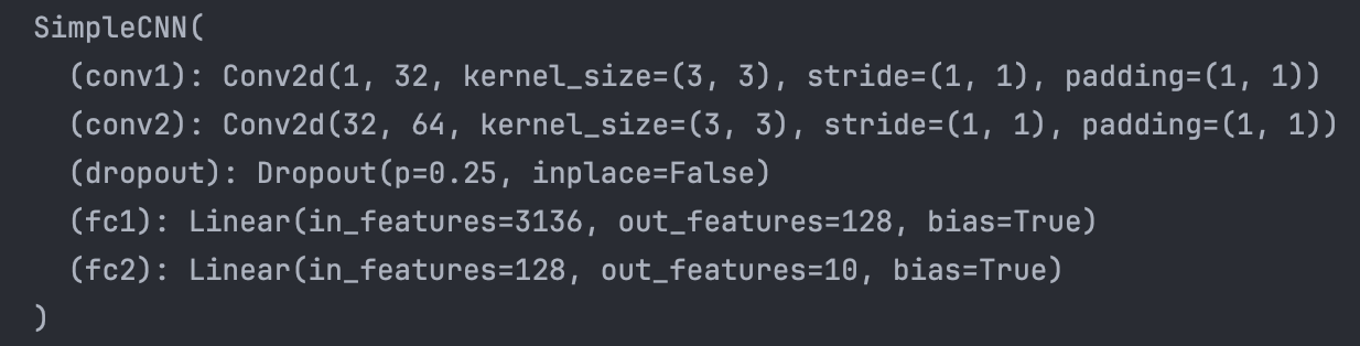

• PyTorch 모델의 학습 시에는 train() 모드를, 예측 시에는 eval() 모드를 구분하여 사용해야 함
• train() 모드에서는 가중치가 정상 업데이트되며 Dropout, Batch Normalization이 정상 동작함
• eval() 모드에서는 가중치가 업데이트 되지 않고 Dropout, Batch Normalization이 비활성화되어 단순히 예측만 수행하게 됨

import numpy as np
import torch.optim as optim
opt = optim.SGD(model.parameters(), lr=0.03)

# PyTorch의 경우 별도 학습과정 지표 저장기능 제공하지 않아 수기 저장 필요함
epoch_train_loss = list()
epoch_train_acc = list()
epoch_test_loss = list()
epoch_test_acc = list()

for epoch in range(10):
    
    # train
    batch_train_loss = list()
    batch_train_acc = list()
    model.train()
    for batch_idx, (im, lbl) in enumerate(train_loader):
        im, lbl = im.to(device), lbl.to(device) # GPU 할당
        opt.zero_grad() # 옵티마이저 초기화
        output = model(im)
        
        loss = F.nll_loss(output, lbl) # F.log_softmax()와 함께 사용 시, One-Hot Encoding 없이 분류 가능
        loss.backward() # 미분 실시
        opt.step() # model.parameters() 자동 업데이트
        batch_train_loss.append(loss.item())
        
        y_pred = output.argmax(dim=1).cpu().numpy()
        y_true = lbl.cpu().numpy()
        acc = np.mean(y_pred == y_true)
        batch_train_acc.append(acc)
        
    epoch_train_loss.append(np.mean(batch_train_loss))
    epoch_train_acc.append(np.mean(batch_train_acc))
    print(f"> [Epoch #{epoch+1} Train] Loss: {np.mean(batch_train_loss):.8f} / Acc: {np.mean(batch_train_acc):.3f}")
        
    # test
    batch_test_loss = list()
    batch_test_acc = list()
    model.eval()
    with torch.no_grad():
        for im, lbl in test_loader:
            im, lbl = im.to(device), lbl.to(device)
            output = model(im)

            loss = F.nll_loss(output, lbl)
            batch_test_loss.append(loss.item())

            y_pred = output.argmax(dim=1).cpu().numpy()
            y_true = lbl.cpu().numpy()
            acc = np.mean(y_pred == y_true)
            batch_test_acc.append(acc)
            
    epoch_test_loss.append(np.mean(batch_test_loss))
    epoch_test_acc.append(np.mean(batch_test_acc))
    print(f"> [Epoch #{epoch+1} Test] Loss: {np.mean(batch_test_loss):.8f} / Acc: {np.mean(batch_test_acc):.3f}")
# > [Epoch #1 Train] Loss: 0.04516698 / Acc: 0.986
# > [Epoch #1 Test] Loss: 0.03436899 / Acc: 0.989
# > [Epoch #2 Train] Loss: 0.04411280 / Acc: 0.986
# > [Epoch #2 Test] Loss: 0.03383952 / Acc: 0.988
# > [Epoch #3 Train] Loss: 0.04298282 / Acc: 0.987
# > [Epoch #3 Test] Loss: 0.03361477 / Acc: 0.988
# > [Epoch #4 Train] Loss: 0.04076239 / Acc: 0.988
# > [Epoch #4 Test] Loss: 0.03141384 / Acc: 0.989
# > [Epoch #5 Train] Loss: 0.04064617 / Acc: 0.988
# > [Epoch #5 Test] Loss: 0.03197801 / Acc: 0.989
# > [Epoch #6 Train] Loss: 0.03836631 / Acc: 0.988
# > [Epoch #6 Test] Loss: 0.03232415 / Acc: 0.989
# > [Epoch #7 Train] Loss: 0.03807409 / Acc: 0.988
# > [Epoch #7 Test] Loss: 0.02985807 / Acc: 0.990
# > [Epoch #8 Train] Loss: 0.03677119 / Acc: 0.989
# > [Epoch #8 Test] Loss: 0.03181267 / Acc: 0.989
# > [Epoch #9 Train] Loss: 0.03529926 / Acc: 0.989
# > [Epoch #9 Test] Loss: 0.02927555 / Acc: 0.989
# > [Epoch #10 Train] Loss: 0.03513584 / Acc: 0.989
# > [Epoch #10 Test] Loss: 0.02880389 / Acc: 0.990

2-3. Evaluation

• 학습과정 확인

fig, ax1 = plt.subplots(figsize=(5, 3))
ax2 = ax1.twinx() # 이중축 설정
ax1.plot(np.arange(1, 11, 1), epoch_train_loss, label="Loss", c="grey")
ax1.set_xlabel("Epoch")
ax1.set_ylabel("Loss")
ax2.plot(np.arange(1, 11, 1), epoch_train_acc, label="Acc.", c="red")
ax2.set_ylim([0.98, 1])
ax2.set_ylabel("Acc.")
fig.suptitle("Loss and Accuracy")
fig.legend(bbox_to_anchor=(0.88, 0.7))
plt.show()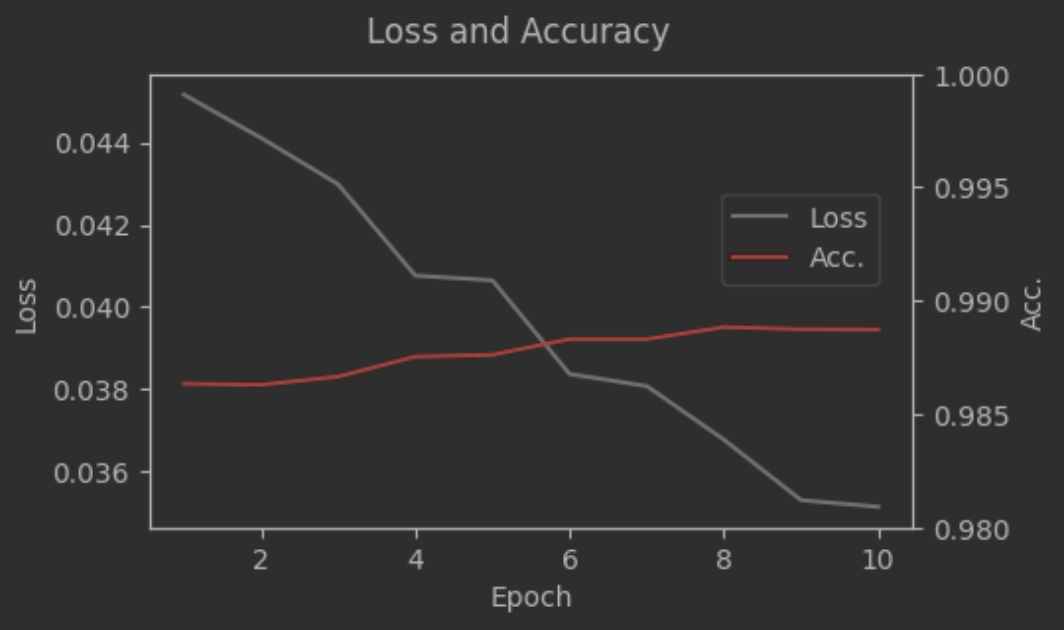

• 후처리

y_true = list()
y_pred = list()
model.eval()
with torch.no_grad():
    for test_im, test_lbl in test_loader:
        test_im, test_lbl = test_im.to(device), test_lbl.to(device)
        test_output = model(test_im)
        y_true.extend(test_lbl.cpu().numpy()) # 실제값
        y_pred.extend(test_output.argmax(dim=1).cpu().numpy()) # 예측값
        
print(y_true[0]) # 7
print(y_pred[0]) # 7

im, lbl = next(iter(test_loader))
plt.figure(figsize=(2,2))
plt.imshow(torch.squeeze(im[0]), cmap="grey")
plt.show()

---

*이 글은 제로베이스 데이터 취업 스쿨의 강의 자료 일부를 발췌하여 작성되었습니다.