강의 내용 복습
(07강) Advanced Object Detection 1
1. Cascade RCNN
1.1 Contribution
faster r-cnn에서 positive/negative sample을 나누는 기준에 대해 고민함
faster r-cnn backbone : 0.7 | head : 0.5
-
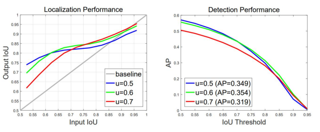
Localization performance
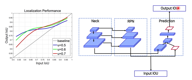
input iou : rpn 통과했을 때 나온 box와 GT의 iou
output iou : head 통과했을 때 나온 box와 GT의 iou
결과 : input iou가 높을수록 높은 IOU threshold에서 학습된 model이 더 좋은 성능을 냄 -
detection performance
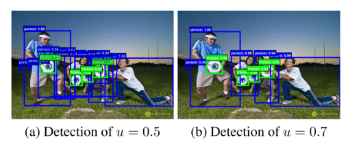
iou threshold : GT와의 iou일 때 u를 기준으로 T/F를 나눔
전반적인 AP의 경우 iou threshold 0.5로 학습된 모델의 성능이 가장 좋지만
AP의 iou threshold가 높아질수록 (AP70, AP90) IoU threshold가 0.6, 0.7로 학습된 모델과 성능 차이가 나지 않음
결론
- 학습되는 IoU에 따라 대응 가능한 IoU 박스가 다름 (낮게 학습했으면 iou낮은 애들 잘 탐지, vice versa)
- 그래프와 같이 high quality detection을 수행하기 위해선 IoU threshold를 높여 학습할 필요가 있음
- 단, 성능이 하락하는 문제가 존재 (iou가 낮을 때)
- 이를 해결하기 위해 Cascade RCNN을 제안
1.2 Method
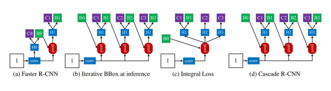
(a) Faster R-CNN
C, B, H0, H1 : classification head , box head , RPN결과 proposal, poolong 결과 fixed feture
C0: 배경ㅇ인지 아닌지만 예측 / C1 : 어떤 object인지까지 예측
(b) Iterative
B0가 아닌 다른 박스가 존재한다면 그 박스로 ROI Pooling진행
head에서 예측된 bbox를 다시 pooling에 이용하는 방법
(c) Integal Loss

- Fastern RCNN과는 다르게 IOU threshold가 다른 Classifier C1, C2, C3를 학습
- Loss의 경우 각각 C1, C2, C3의 classifier loss를 합
- Inference 시, C1, C2, C3의 confidence 를 평균 냄
- 큰 성능 향상은 없음
(d) Cascade R-CNN
- 여러 개의 RoI head (H1, H2, h3)를 학습
- 이 때 Head 별로 IOU threshold를 다르게 설정
- C3, B3가 최종 결과
결과


- Bbox pooling을 반복 수행할 시 성능 향상되는 것을 증명 (Iterative)
- IOU threshold가 다른 Classifier가 반복될 때 성능 향상 증명 (Integral)
- IOU threshold가 다른 RoI head를 cascade로 쌓을 시 성능 향상 증명 (Cascade)
2. Deformable Convolutional Networks (DCN)
2.1 Contribution
CNN 문제점 : 일정한 패턴을 지닌 convolution neural networks는 geometric transformations(Affine, view point, Pose 변화)에 한계를 지님
기존 해결 방법 : Geometric augmentation, Geometric invariant feature engineering
Geometric invariant feature selection
사람이 생각하지 못하는 feature는 모델이 학습하지 못하는 단점
2.2 Method
Deformable Convolution
이미지에 사람은 이해하지 못하지만 computer는 이해하는 geometric 연산을 스스로 찾아 conviution filter size를 변형할 수 있게 하는 것이 main idea
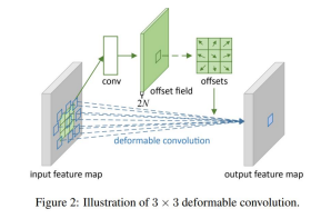

(a) : vanilla conv
(b),(c),(d) : offset(= geometric transform)을 추가해서 kernel위치에서 offset만큼 이동한 image pixel과 곱하도록 함
- 일반적인 convolution을 offset으로 표현했을때
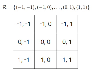
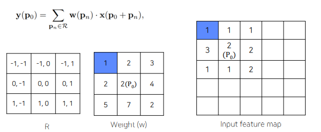 p0을 기준으로 R의 각 pixel에 해당하는 offset만큼 이동한 후 이미지와 곱하면 됨.
이 R의 pixel값을 다르게 바꾸면 Deformable Convolution
한 점 𝑃0 에 deformable convolution layer
∆𝑃𝑛 만큼 더해줌으로써 deformable 하게 만들어줌.
 객체가 있을 법한 위치에서 convoution을 수행
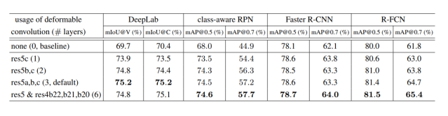
결론
- 일정한 패턴을 지닌 convolution neural networks는 geometric transformations에 한계를 파악
- 일정한 패턴이 아니라 offset을 학습시켜 위치를 유동적으로 변화
- 주로 object detection, segmentation에서 좋은 효과를 보임
3. Transformer
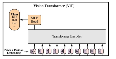
3.1 Vision Transformer (ViT)
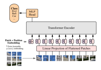
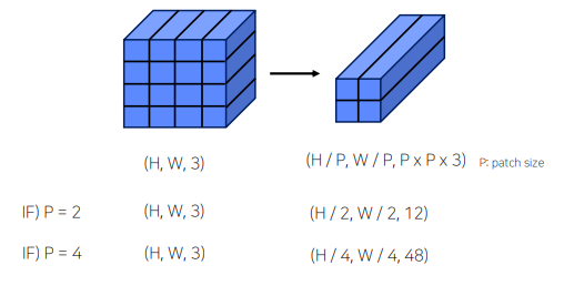
1) Flatten 3D to 2D (Patch 단위로 나누기)
 P = PATCH 크기 , N = , Reshape image :
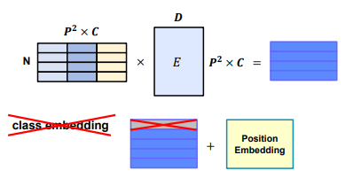
2) Learnable한 embedding 처리
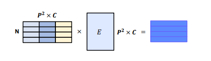 E 라는 matrix를 이용해서 학습을 가능하게 만들어줌
3) Add class embedding, position embedding
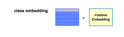 앞서 만들어진 embedding 값에 class embedding 추가 ([CLS]Token) , 이미지의 위치 따라 학습하기 위해 position embedding 추가
4) Transformer
 Embedding: Transformer 입력값
5) Predict
Class embedding vector 값을 MLP head에 입력시켜 최종 결과를 추출
문제점
- ViT의 실험부분을 보면 굉장히 많은양의 Data를 학습하여야 성능이 나옴
- Transformer 특성상 computational cost 큼
- 일반적인 backbone으로 사용하기 어려움
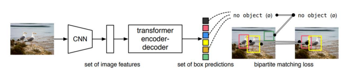
3.2 End-to-End Object Detection with Transformer
- Transformer를 처음으로 Object Detection에 적용
- 기존의 Object Detection의 hand-crafted post process 단계를 transformer를 이용해 없앰
Prediction Head
 기존에는 NMS를 통해 box 선택
architecture
Encoder
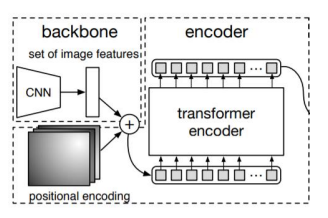
Transformer 특성상 많은 연산량이 필요하여 highest level feature map만 사용
Flatten 2D
Positional embedding
Encoder
224 x 224 input image
7 x 7 feature map size
49 개 의 feature vector 를 encoder 입력값으로 사용
Decorder

Decoder
Feed Forward Network (FFN)
N개의 output
이 때 N은 한 이미지에 존재하는 object 개수보다 높게 설정
Train
- 이 때 groundtruth에서 부족한 object 개수만큼 no object로 padding 처리
- 따라서 groundtruth와 prediction이 N:N 매핑
- 각 예측 값이 N개 unique하게 나타나 post-process 과정이 필요 없음
결과
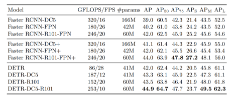
전체적인 AP는 상승하였으나, highest level feature만 사용하여 하락
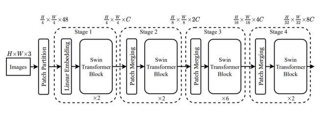
3.3 Swin Transformer
- transformer 를 backbone으로 사용
- CNN과 유사한 구조로 설계
- Window라는 개념을 활용하여 cost를 줄임
Architecture
-
Patch Partitioning
-
Linear Embedding
-
Swin Transformer Block

2번의 attention -> window-multi head self attention / shifted window-multi head self attention -
Window Multi-head Attention

Window 단위로 embedding을 나눔.
기존 ViT같은 경우 모든 embedding을 Transformer에 입력
Swin-Transformer는 Window 안에서만 Transformer 연산 수행
따라서 이미지 크기에 따라 증가되던 computational cost가 Window 크기에 따라 조절 가능
Window 안에서만 수행하여 receptive field를 제한하는 단점 존재 -
shifted window-multi head self attention
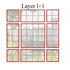
W-MSA의 경우 Window 안에서만 수행하여 receptive field를 제한하는 단점 존재
이를 해결하기 위해 Shifted Window Multi-Head Attention을
Transformer Block 2번째 layer에서 수행
Window size와 다르게 나뉜 부분들 해결 필요
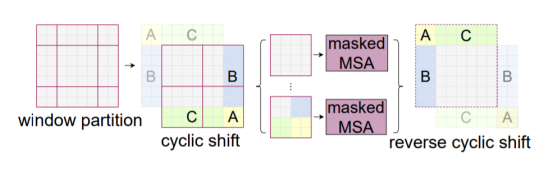
남는 부분들 (A, B, C)를 그림과 같이 옮겨줌
이 때 남는 부분들을 masking 처리하여 self-attention 연산이 되지 않도록 함 -
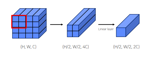
Patch Merging
결과
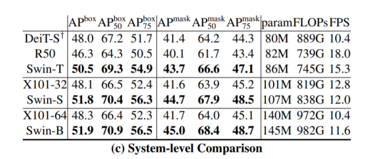
- 적은 Data에도 학습이 잘 이루어짐
- Window 단위를 이용하여 computation cost를 대폭 줄임
- CNN과 비슷한 구조로 Object Detection, Segmentation 등의 backbone으로 general하게 활용
Further Reading
Cascade R-CNN: High Quality Object Detection and Instance Segmentation
Deformable Convolutional Networks
Swin Transformer: Hierarchical Vision Transformer using Shifted Windows
과제 수행 과정 및 결과
피어 세션
학습 회고