모두를 위한 딥러닝 - ML Lec 07

Dylan·2022년 8월 2일

모두를위한딥러닝

모두를 위한 딥러닝

목록 보기

7/12

lec 07-1: 학습 rate, Overfitting, 그리고 일반화 (Regularization)

Gradient descent

우리가 cost function을 정의하고 그 cost function을 최소화하는 값을 찾기 위해서 사용 했던 Gradient descent 알고리즘 이다.

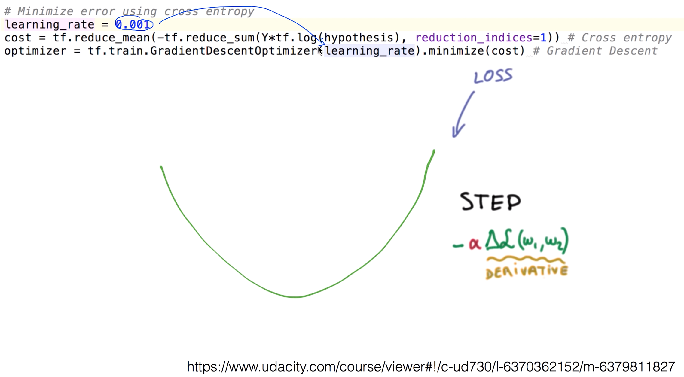
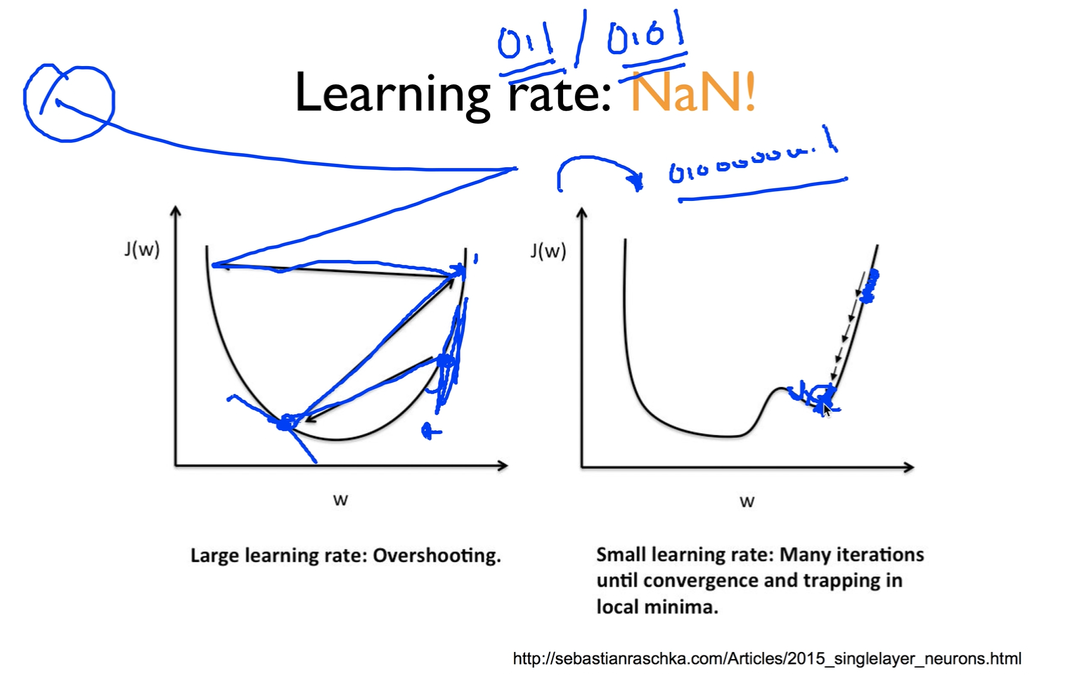
Large learning rate : overshooting

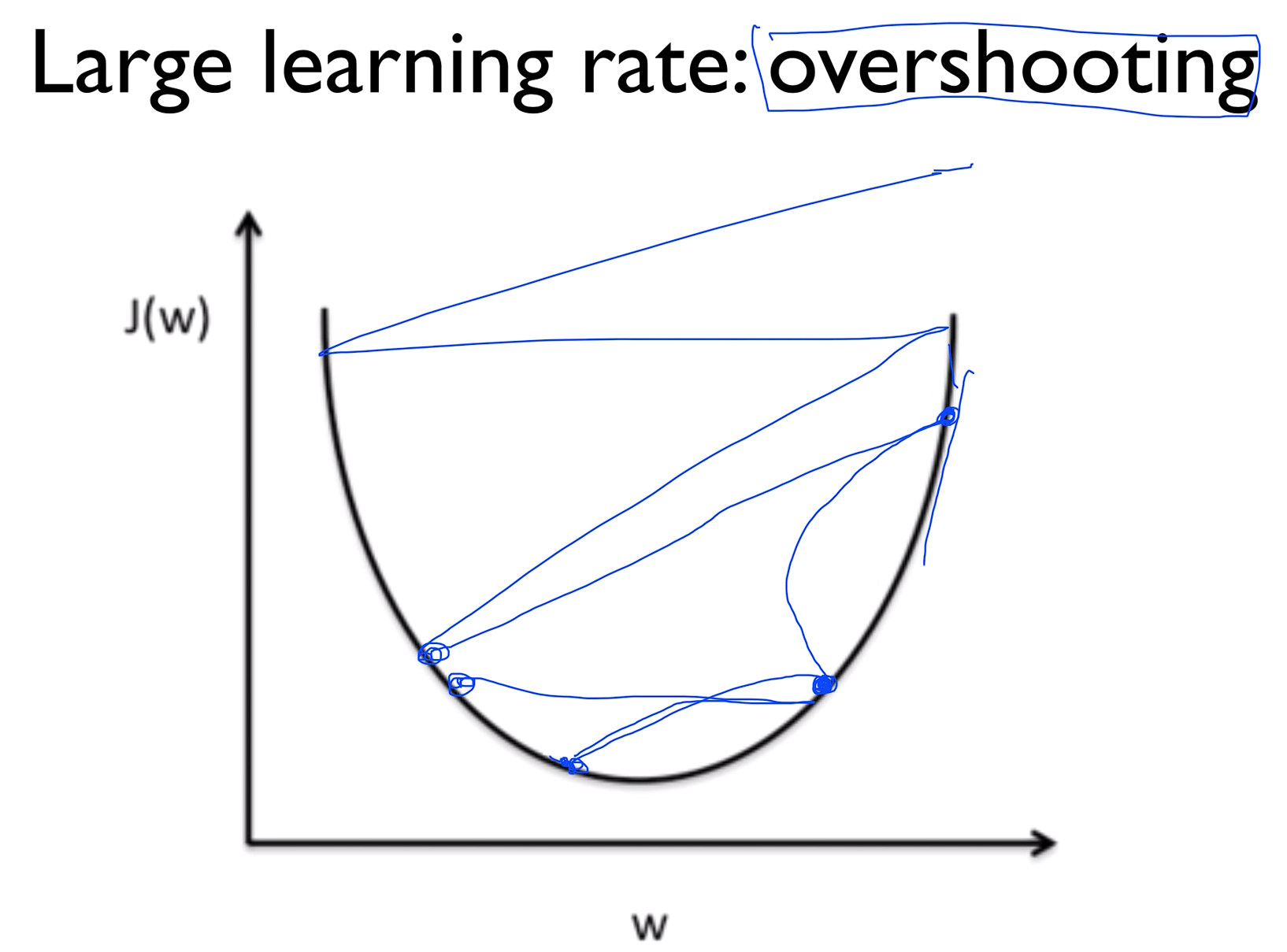
러닝 레이트를 잘 정하는게 중요한데 만약에 이 값을 엄청 크게 주었다고 가정해 보자.
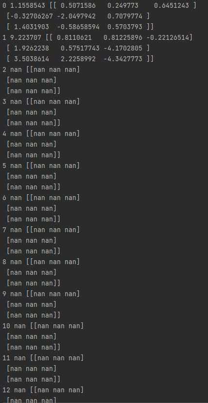
그럴 땐 그래프 바깥으로 튕겨나가버릴 수 있다. 이렇게하면 학습이 이루어지지 않을 뿐만 아니라 코스트펑션을 출력할 때 숫자가 아닌 값들이 찍혀나올 수 있다. 이러한 현상을 Overshooting 이라 한다.

Small learning rate : takes too long, stops at local minimum

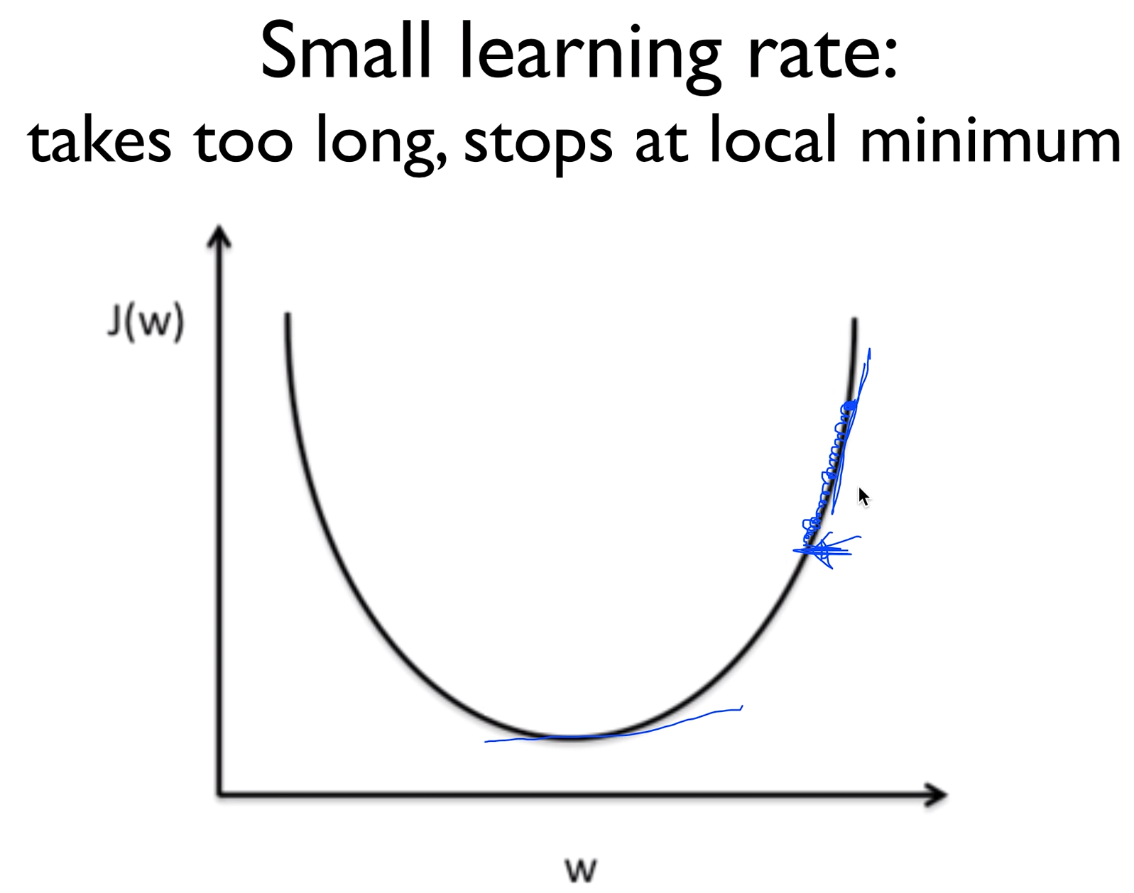
반대로 굉장히 작은 러닝 레이트를 지정해준다면 지정한 횟수를 수행하고도 최저점을 못찾고 중간에 멈춰버릴 수 있다.

Try several learning rates

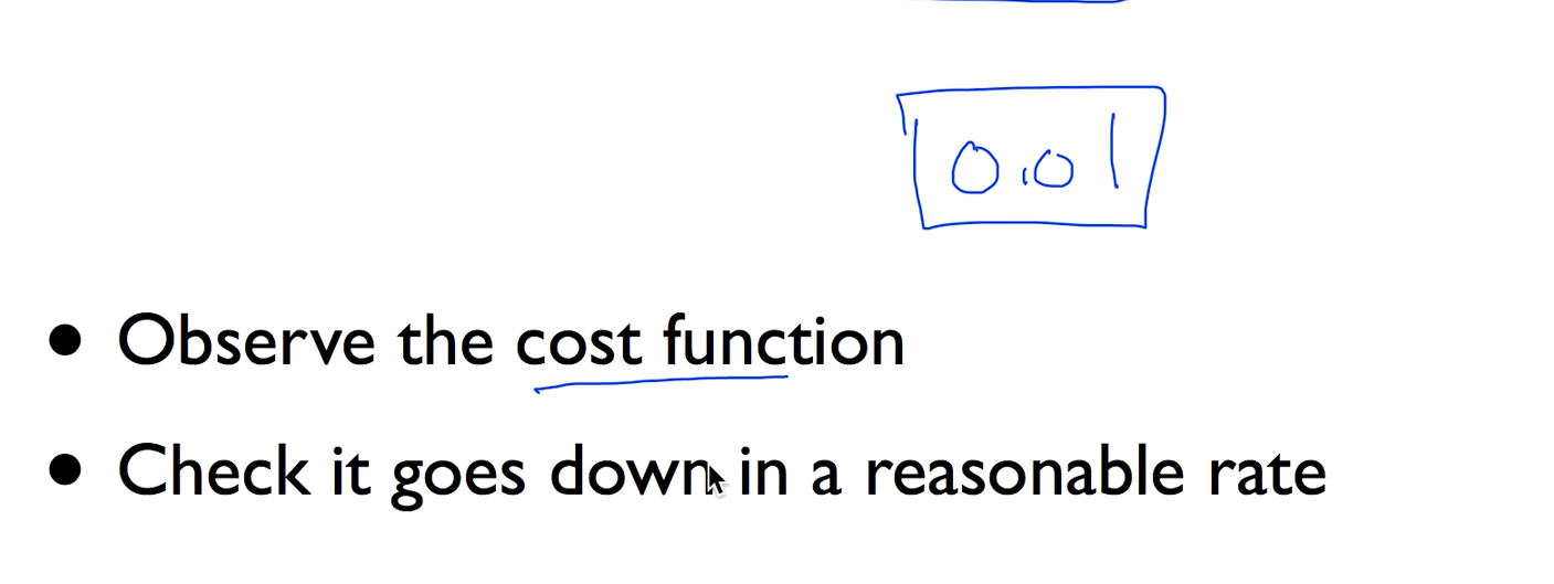
전반적으로는 러닝 레이트를 정하는 것에 특별한 방법은 없다.가진 환경에 따라 다 다르기 때문에 보통 0.01로 시작을 많이 하고 오버슈팅이 일어나면 작게 반대로 너무 적게 움직여서 끝나는거같으면 크게 올리면 된다.

Data (X) preprocessing for gradient descent

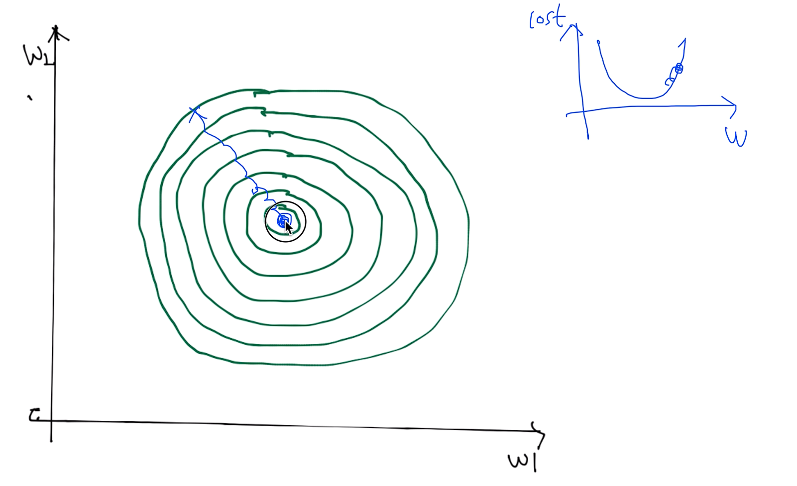
데이터를 사전처리해야할 이유가 있는데, 우리가 가장 많이 사용하는 알고리즘인 gradient descent 알고리즘으로 예시를 들겠다.

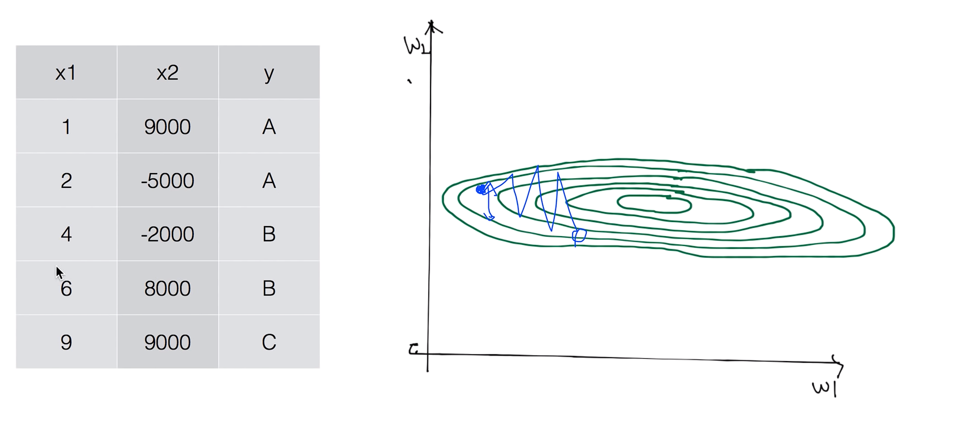
예를 들어서 우리가 가지고 있는 데이터의 값 중에 x1의 값과 x2의 값에 큰 차이가 난다면 이전 그래프의 등고선 모양보다는 옆으로 길게 늬운 등고선이 나타난다.
그러면 우리가 시작점을 잡고 러닝 레이트 값이 좋은 값임에도 불과하고 조금이라도 밖으로 나가게되면 튀어 나가게 되어버린다.
데이터 값에 큰 차이가 있을 경우에 Normalize 할 필요가 있다

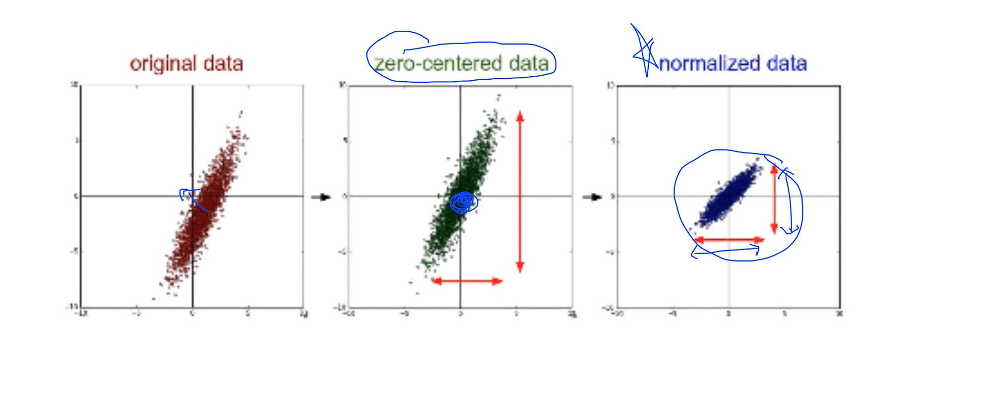
오리지날 데이터가 2차원 형태로 저렇게 되어 있다고 할 때 보통 많이 쓰는 방법이 zero-centered data이며 데이터의 중심이 0으로 갈 수 있도록 바꿔주는 방법을 취하기도 하고
또 가장 많이 사용하는 방법은 어떤 값이 이 값 전체의 범위가 어떤 형태의 범위안에 항상 들어가도록 Normalized data 하는 방법이 있다

그래서 내가 러닝 레이트를 잘 잡은 거 같은데 이상하게 학습이 일어나지 않고 코스트 함수가 발산을 한다거나 이상한 동작을 보일때는 데이터중에 큰 차이가 나는 값이 있는지 그리고 preprocessing을 했는지 점검해보면 좋다

Standardization

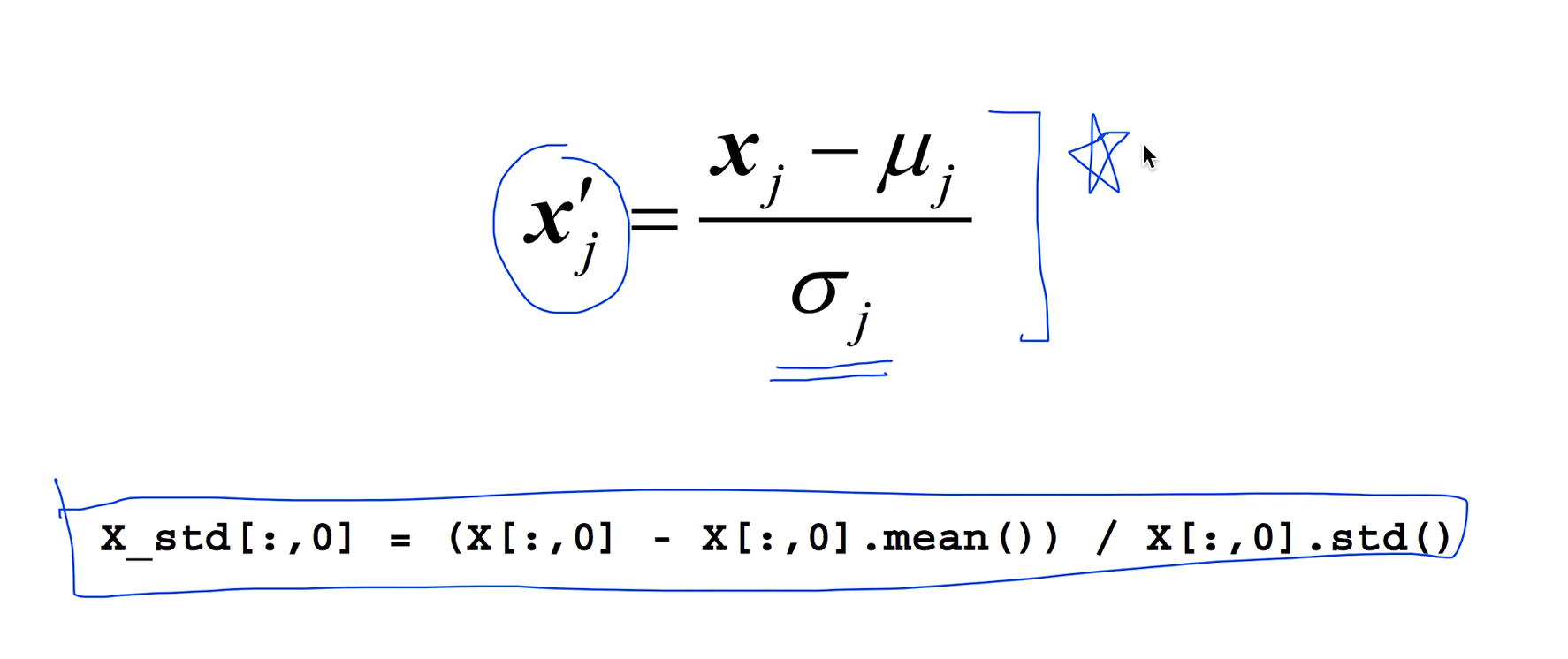
x의 값을 우리가 계산한 평균과 분산의 값을 가지고 나누어 주면 되는데 파이썬을 가지고 만든다면 이렇게 한줄로 표시할 수 있다.
이런 형태의 노말리제이션이 있지만 그 중에 한 가지를 선택해서 x 데이터를 처리해보는 것도 머신러닝에 좋은 성능을 발휘하기 위한 방법일 수가 있다.

Overfitting

Our model is very good with training data set (with memorization)
Not good at test dataset orin real use

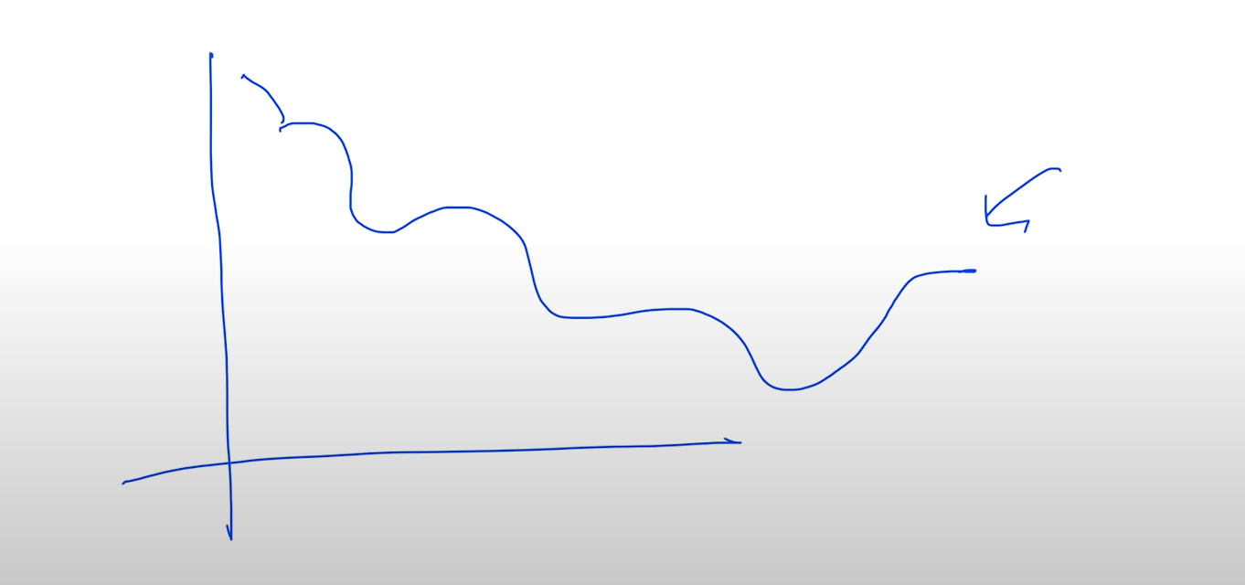
머신러닝의 가장 큰 문제인 Overfitting, 오버피팅이란 학습 데이터에 너무 잘맞는 모델을 만들 수가 있는데 training data set에는 잘 맞지만 test data set이나 실제 사용했을 경우에는 정확성이 떨어지는걸 오버피팅이라 한다

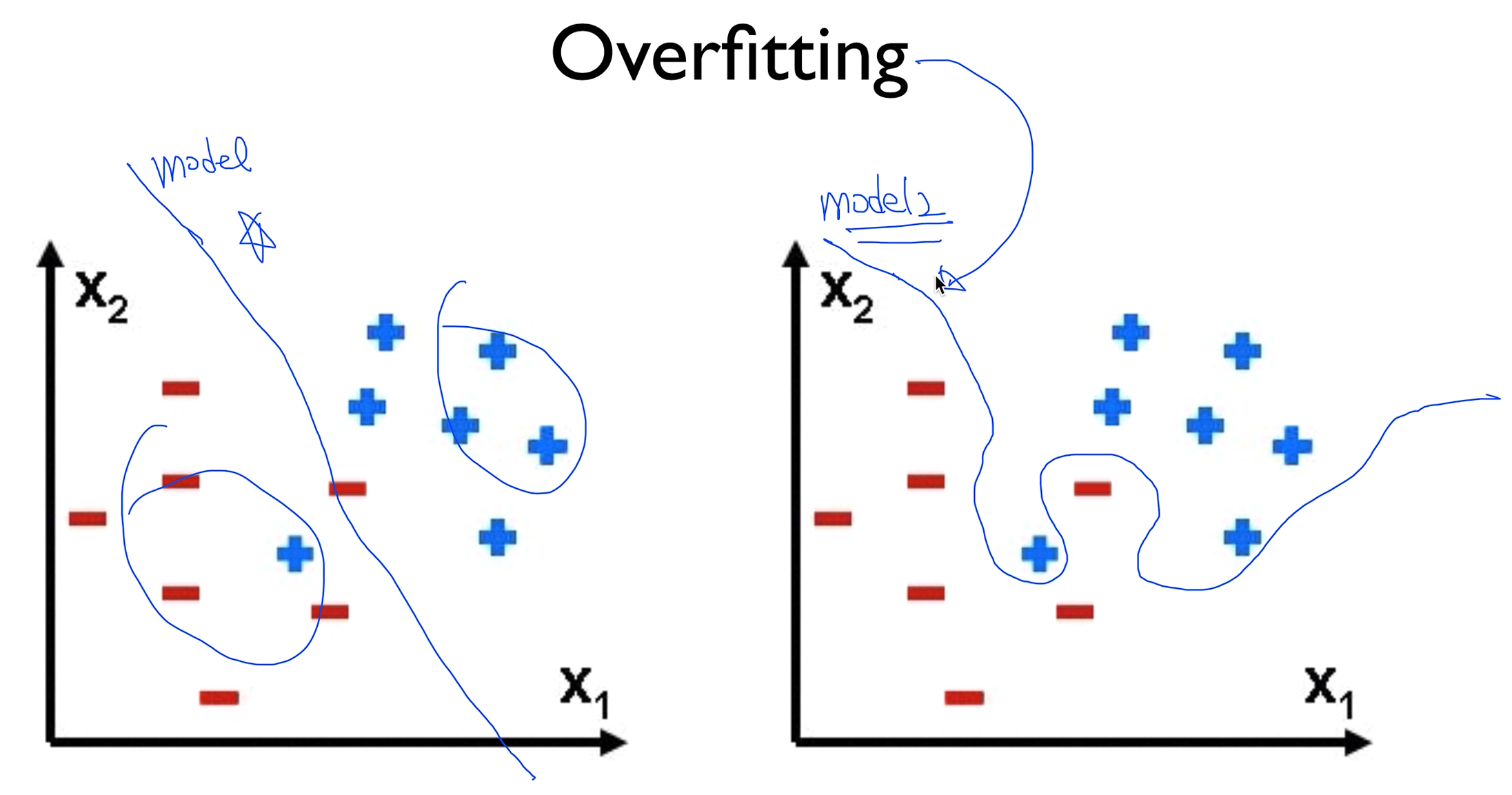
왼쪽 모델1같은 경우는 리니어하게 그어서 좋은 모델의 표본이라 할 수 있지만
오른쪽 모델2같은 경우는 가지고 있는 데이터에 너무 딱 맞게 선을 그어버려서 training data set에는 잘 맞겠지만 다른 데이터가 들어오게 될 때는 굉장히 정확도가 떨어 질 수 있다. 이러한 모델이 오버피팅이다.

Solutions for overfitting

More training data!
Reduce the number of features
Regularization

오버피팅을 줄이는 가장 좋은 방법은 training data를 많이 가지고 있는것이다
또 하나는 우리가 가지고 있는 features의 갯수를 중복된 것이 있으면 줄인다던지 이런 방법도 오버피팅을 줄이는방법이다.

마지막으로 이 두가지 방법 외에도 하나의 기술적인 방법이 있는데 이게 Regularization이라는 방법이다.

Regularization

Let's not have too big numbers in the weight

일반화 시킨다는 얘기는 우리가 가지고 있는 w를 너무나 큰 값을 가지지 말자
우리가 주로 오버피팅이라고 설명을 할 때 보통 그래프의 선을 데이터에 맞게 구부리는 것을 말하는데 이것을 구부리지말고 피자 라고 하는걸 Regularization
여기서 편다는 이야기는 같이 좀 w이 적은 값을 가진다는 얘기고 구부린다는 것은 w값이 큰 값을 가졌을때 구부러지는건데 그래서 좀 구부리지 말고 좀 펴 라는 얘기이다.

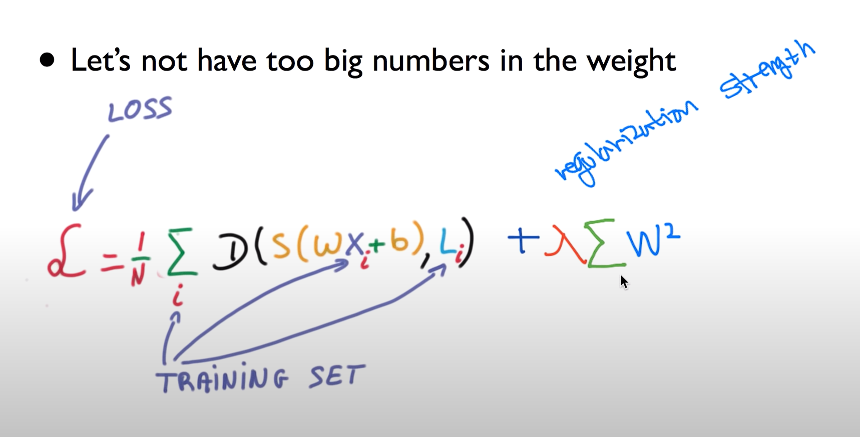
이것을 하기 위해서는 우리가 코스트 함수를 설명할 때 코스트를 최소화 시키는 것이 우리의 목표였는데 이 코스트 함수의 뒤에 이 텀을 추가시켜 준다

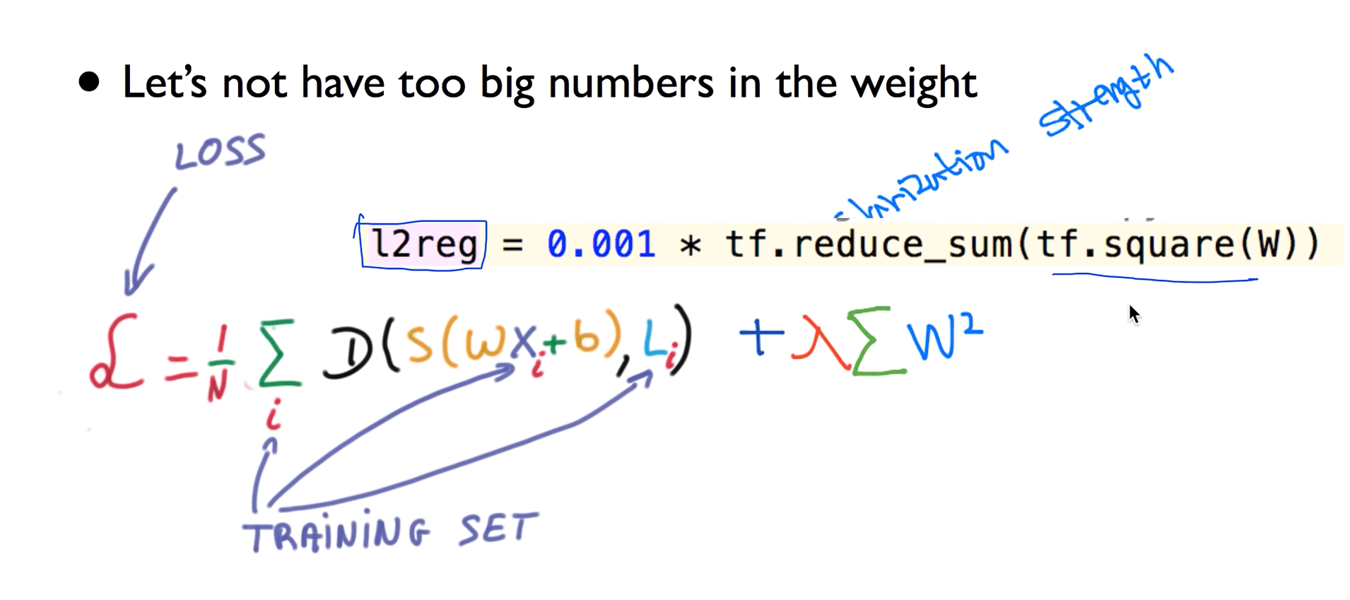
람다값을 regularization strength라 한다
텐서플로우로 구현할때 간단하게 표현할 수 있다.

lec 07-2: Training/Testing 데이타 셋

Performance evaluation: is this good?

이전 시간에 배운것들을 통해서 우리의 머신러닝 모델을 데이터를 가지고 학습을 시켰다.
이렇게 학습을 시킨 모델이 얼마나 훌륭한가? 얼마나 성공적으로 예측을 할 수 있을까 평가를 할까요

Evaluation using training set?

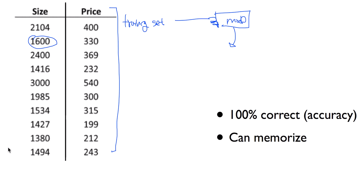
우리가 이런 형태의 데이터가 있다고 생각을 해보자. 보통 training set 을 가지고 모델을 학습을 시키는데 다 시키고 난 뒤 다시 training set 을 가지고 물어보게 되면 이것이 공정한 방법일까요? 이런식으로 한다면 머신러닝은 100% 완벽한 답을 할 수도 있을것이다. 그냥 외워버리면 되니까
이것은 좋은방법이 아니다

Training and test sets

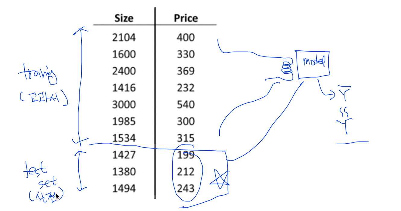
좋은 방법은 우리가 시험을 보는 방식이랑 똑같다. 얼추 3:7로 나뉘어서 7은 training 3은 test set으로 구분해서 training set을 가지고 모델을 학습 시키고 완벽하게 끝났다라고 했을 때 단 한번의 기회로 testing data set을 가지고 비교를 한다.
한마디로 training set은 교과서이고 이 교과서를 가지고 공부를 하다가 다 했을 경우 testing data set을 시험이라 비유했을 경우 단 한번 시험으로 성능을 평가하면 된다.

Training, validation and test sets

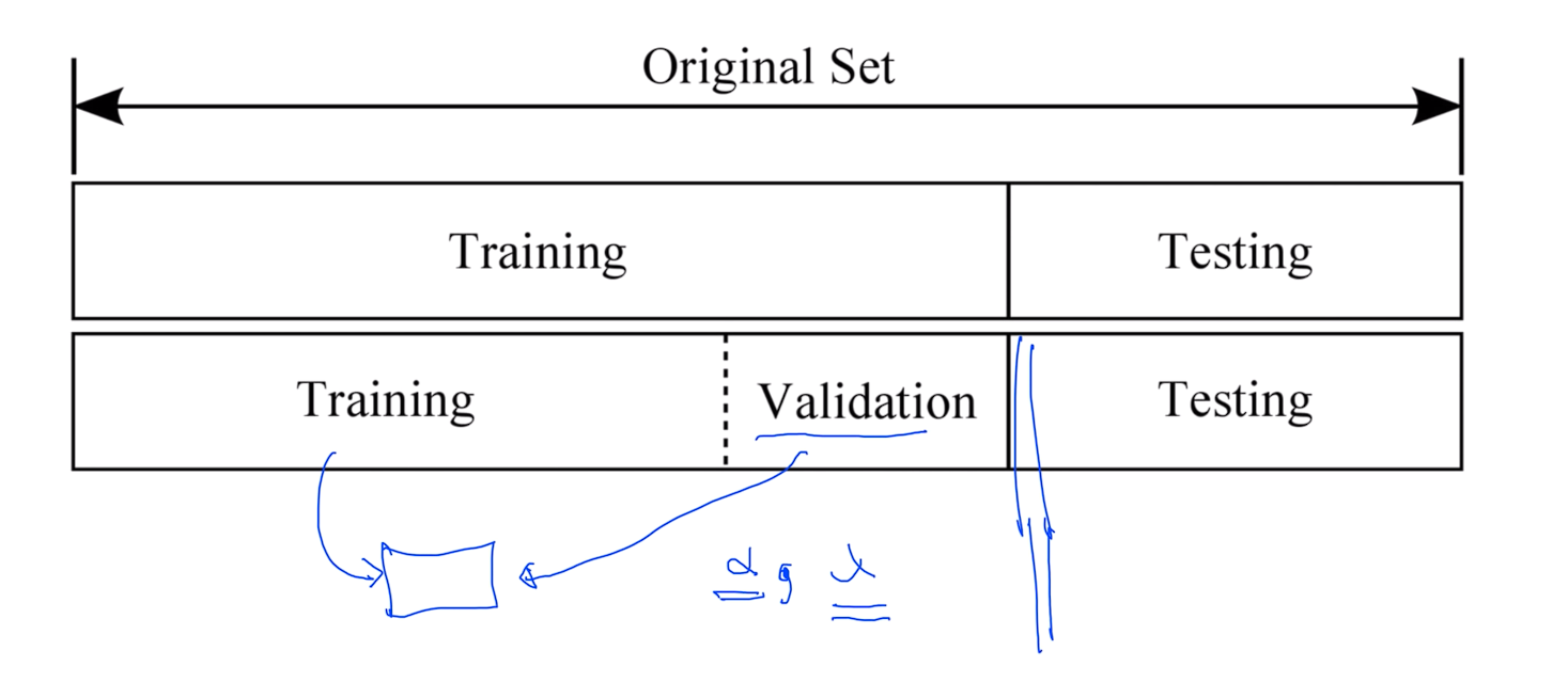
바로 직전에 얘기 했듯이 보통 통상적으로 트레이닝 셋과 테스팅 셋으로 나뉘는게 일반적인데
지난번에 얘기 할때 알파라는 러닝 레이트라는것을 얘기 했었고, 또 하나의 상수가 학습할 때 들어가는 것이 람다라고 했던 어떤 레귤러제이션을 하는데 얼마나 강하게 할것인가하는 값이였다.
이러한 값을 조금 튜닝할 필요가 있을 때 우리가 가지고 있는 트레이닝 셋을 Training과 Validation 두개로 다시 나눕니다.
일반적으로 트레이닝 셋으로 모델을 학습시킨 다음에 이 벨리데이션 셋을 가지고 이런 상수 값들이 어떤것이 좋을까 하는 것들을 튜닝을 하게 된다. 이것을 이제 Validation이라 하고 비유하자면 모의고사로 보면 되고 해서 완벽하게 되면 이제 Testing data set을 가지고 모델이 잘 동작하는지 평가를 하면 된다.

Online learning

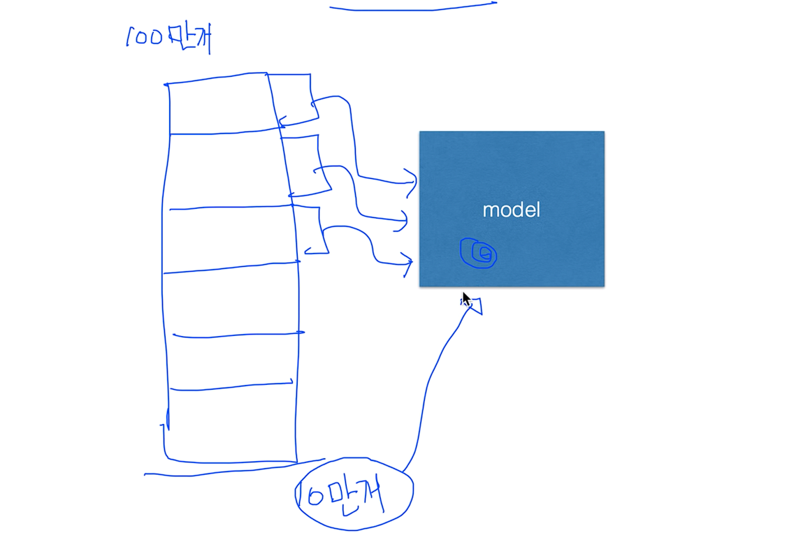
그리고 데이터 셋이 굉장히 많을 경우에 한번에 다 넣어서 학습을 시키기가 힘들 때가 있다.
이럴 때 나온게 Online learning이다.

예를 들어 데이터가 100만개가 있다고 가정할때, 한번에 넣어서 학습을 시킬려면 베타공간도 많이 필요하고 하니까 그렇게 하지 않고 잘라 가지고 10만개 씩 잘라서 학습을 시킵니다. 한번 학습 시키고 끝났으면 두번째를 학습시키고 세번째를 학습시키고,, 자 이때 모델이 해야하는 일은 첫번째 학습이 된 결과가 모델에 남아 있어야 한다. 그래서 두번째 데이터를 학습 시키면 이 모델에 추가가 되어서 새로운 학습이 되어야 한다.

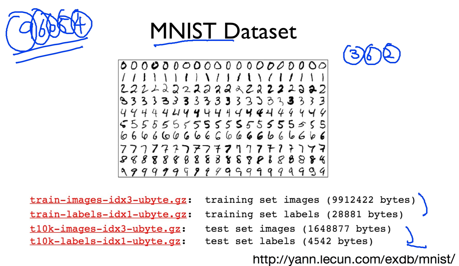
MINIST Dataset

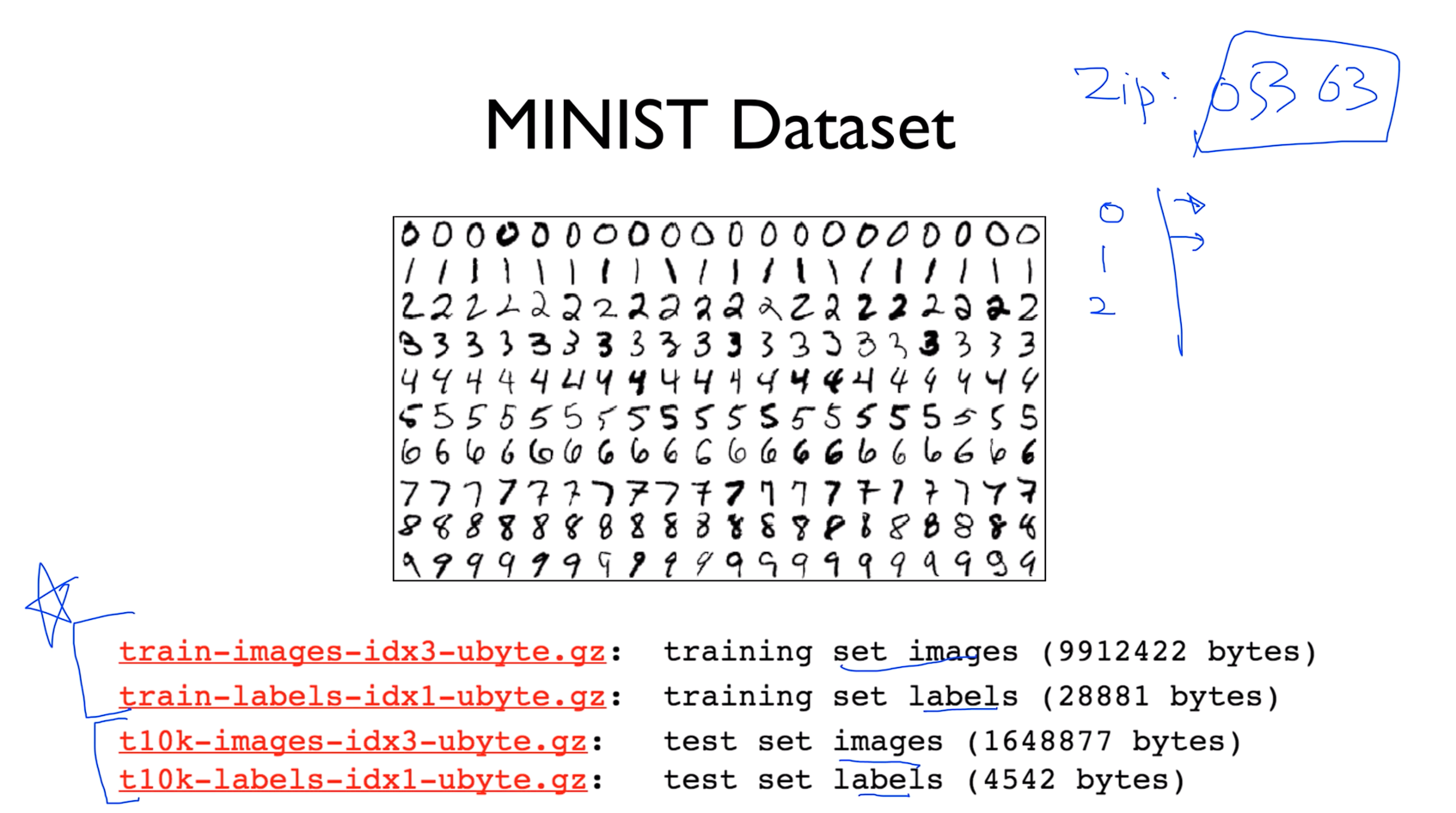
유명한 데이터셋인데 그림을 보면 사람이 적어놓은 숫자를 컴퓨터가 인식을 할 수 있는지를 테스트하는 Dataset 이다. 이것이 필요했던 이유는 미국 우체국에서 우편번호를 받게되면 최소한 자동으로 분류를 할 수 있게 컴퓨터에게 시키기 위해서 만들어졌다.

여기 보면 데이터셋이 나뉘어져 있는데 training set과 test set으로 나뉘어져있는것을 볼 수 있다.

ML lab 07-1: training/test dataset, learning rate, normalization

Training and Test datasets

import tensorflow.compat.v1 as tf
tf.disable_v2_behavior()

tf.set_random_seed(777)  # for reproducibility

x_data = [[1, 2, 1], [1, 3, 2], [1, 3, 4], [1, 5, 5], [1, 7, 5], [1, 2, 5], [1, 6, 6], [1, 7, 7]]
y_data = [[0, 0, 1], [0, 0, 1], [0, 0, 1], [0, 1, 0], [0, 1, 0], [0, 1, 0], [1, 0, 0], [1, 0, 0]]

# Evaluation our model using this test dataset
x_test = [[2, 1, 1], [3, 1, 2], [3, 3, 4]]
y_test = [[0, 0, 1], [0, 0, 1], [0, 0, 1]]

X = tf.placeholder("float", [None, 3])
Y = tf.placeholder("float", [None, 3])

W = tf.Variable(tf.random_normal([3, 3]))
b = tf.Variable(tf.random_normal([3]))

# tf.nn.softmax computes softmax activations
# softmax = exp(logits) / reduce_sum(exp(logits), dim)
hypothesis = tf.nn.softmax(tf.matmul(X, W) + b)

# Cross entropy cost/loss
cost = tf.reduce_mean(-tf.reduce_sum(Y * tf.log(hypothesis), axis=1))
# Try to change learning_rate to small numbers
optimizer = tf.train.GradientDescentOptimizer(learning_rate=0.1).minimize(cost)

# Correct prediction Test model
prediction = tf.argmax(hypothesis, 1)
is_correct = tf.equal(prediction, tf.argmax(Y, 1))
accuracy = tf.reduce_mean(tf.cast(is_correct, tf.float32))

# Launch graph
with tf.Session() as sess:
    # Initialize TensorFlow variables
    sess.run(tf.global_variables_initializer())

    for step in range(201):
        cost_val, W_val, _ = sess.run([cost, W, optimizer], feed_dict={X: x_data, Y: y_data})
        print(step, cost_val, W_val)

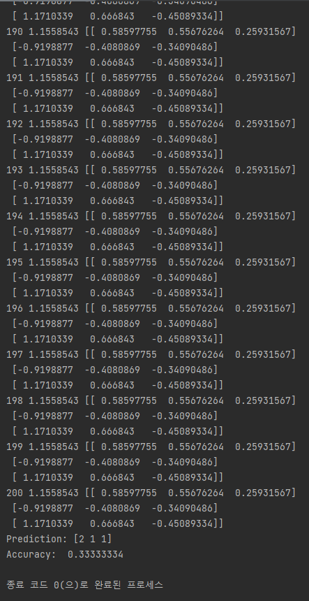
    # predict
    print("Prediction:", sess.run(prediction, feed_dict={X: x_test}))
    # Calculate the accuracy
    print("Accuracy: ", sess.run(accuracy, feed_dict={X: x_test, Y: y_test}))

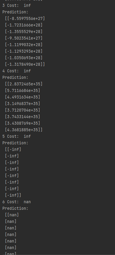
Learning rate: NaN!

Big learning rate - ex) 1.5 일 때

import tensorflow.compat.v1 as tf
tf.disable_v2_behavior()

tf.set_random_seed(777)  # for reproducibility

x_data = [[1, 2, 1], [1, 3, 2], [1, 3, 4], [1, 5, 5], [1, 7, 5], [1, 2, 5], [1, 6, 6], [1, 7, 7]]
y_data = [[0, 0, 1], [0, 0, 1], [0, 0, 1], [0, 1, 0], [0, 1, 0], [0, 1, 0], [1, 0, 0], [1, 0, 0]]

# 이 테스트 데이터 세트를 사용하여 모델 평가
x_test = [[2, 1, 1], [3, 1, 2], [3, 3, 4]]
y_test = [[0, 0, 1], [0, 0, 1], [0, 0, 1]]

X = tf.placeholder("float", [None, 3])
Y = tf.placeholder("float", [None, 3])

W = tf.Variable(tf.random_normal([3, 3]))
b = tf.Variable(tf.random_normal([3]))

# tf.nn.softmax computes softmax activations
# softmax = exp(logits) / reduce_sum(exp(logits), dim)
hypothesis = tf.nn.softmax(tf.matmul(X, W) + b)

# Cross entropy cost/loss
cost = tf.reduce_mean(-tf.reduce_sum(Y * tf.log(hypothesis), axis=1))
# Try to change learning_rate to small numbers
optimizer = tf.train.GradientDescentOptimizer(learning_rate=1.5).minimize(cost)

# 정확한 예측 테스트 모델
prediction = tf.argmax(hypothesis, 1)
is_correct = tf.equal(prediction, tf.argmax(Y, 1))
accuracy = tf.reduce_mean(tf.cast(is_correct, tf.float32))

# Launch graph
with tf.Session() as sess:
    # 세션을 열고 변수 초기화
    sess.run(tf.global_variables_initializer())

    for step in range(201):
        cost_val, W_val, _ = sess.run([cost, W, optimizer], feed_dict={X: x_data, Y: y_data})
        print(step, cost_val, W_val)

    # 테스트 데이터로 확인해보기
    print("Prediction:", sess.run(prediction, feed_dict={X: x_test}))
    # Calculate the accuracy
    print("Accuracy: ", sess.run(accuracy, feed_dict={X: x_test, Y: y_test}))

Small learning rate - ex) 1e-10 일 때

import tensorflow.compat.v1 as tf
tf.disable_v2_behavior()

tf.set_random_seed(777)  # for reproducibility

x_data = [[1, 2, 1], [1, 3, 2], [1, 3, 4], [1, 5, 5], [1, 7, 5], [1, 2, 5], [1, 6, 6], [1, 7, 7]]
y_data = [[0, 0, 1], [0, 0, 1], [0, 0, 1], [0, 1, 0], [0, 1, 0], [0, 1, 0], [1, 0, 0], [1, 0, 0]]

# 이 테스트 데이터 세트를 사용하여 모델 평가
x_test = [[2, 1, 1], [3, 1, 2], [3, 3, 4]]
y_test = [[0, 0, 1], [0, 0, 1], [0, 0, 1]]

X = tf.placeholder("float", [None, 3])
Y = tf.placeholder("float", [None, 3])

W = tf.Variable(tf.random_normal([3, 3]))
b = tf.Variable(tf.random_normal([3]))

# tf.nn.softmax computes softmax activations
# softmax = exp(logits) / reduce_sum(exp(logits), dim)
hypothesis = tf.nn.softmax(tf.matmul(X, W) + b)

# Cross entropy cost/loss
cost = tf.reduce_mean(-tf.reduce_sum(Y * tf.log(hypothesis), axis=1))
# Try to change learning_rate to small numbers
optimizer = tf.train.GradientDescentOptimizer(learning_rate=1e-10).minimize(cost)

# 정확한 예측 테스트 모델
prediction = tf.argmax(hypothesis, 1)
is_correct = tf.equal(prediction, tf.argmax(Y, 1))
accuracy = tf.reduce_mean(tf.cast(is_correct, tf.float32))

# Launch graph
with tf.Session() as sess:
    # 세션을 열고 변수 초기화
    sess.run(tf.global_variables_initializer())

    for step in range(201):
        cost_val, W_val, _ = sess.run([cost, W, optimizer], feed_dict={X: x_data, Y: y_data})
        print(step, cost_val, W_val)

    # 테스트 데이터로 확인해보기
    print("Prediction:", sess.run(prediction, feed_dict={X: x_test}))
    # Calculate the accuracy
    print("Accuracy: ", sess.run(accuracy, feed_dict={X: x_test, Y: y_test}))

Non-normalized inputs

import tensorflow.compat.v1 as tf
tf.disable_v2_behavior()
import numpy as np
tf.set_random_seed(777)  # for reproducibility


xy = np.array([[828.659973, 833.450012, 908100, 828.349976, 831.659973],
               [823.02002, 828.070007, 1828100, 821.655029, 828.070007],
               [819.929993, 824.400024, 1438100, 818.97998, 824.159973],
               [816, 820.958984, 1008100, 815.48999, 819.23999],
               [819.359985, 823, 1188100, 818.469971, 818.97998],
               [819, 823, 1198100, 816, 820.450012],
               [811.700012, 815.25, 1098100, 809.780029, 813.669983],
               [809.51001, 816.659973, 1398100, 804.539978, 809.559998]])

x_data = xy[:, 0:-1]
y_data = xy[:, [-1]]

# placeholders for a tensor that will be always fed.
X = tf.placeholder(tf.float32, shape=[None, 4])
Y = tf.placeholder(tf.float32, shape=[None, 1])

W = tf.Variable(tf.random_normal([4, 1]), name='weight')
b = tf.Variable(tf.random_normal([1]), name='bias')

# Hypothesis
hypothesis = tf.matmul(X, W) + b

# Simplified cost/loss function
cost = tf.reduce_mean(tf.square(hypothesis - Y))

# Minimize
optimizer = tf.train.GradientDescentOptimizer(learning_rate=1e-5)
train = optimizer.minimize(cost)

# Launch the graph in a session.
sess = tf.Session()
# Initializes global variables in the graph.
sess.run(tf.global_variables_initializer())

for step in range(101):
    cost_val, hy_val, _ = sess.run(
        [cost, hypothesis, train], feed_dict={X: x_data, Y: y_data})
    print(step, "Cost: ", cost_val, "\nPrediction:\n", hy_val)

Normalized inputs (min-max scale)

import tensorflow.compat.v1 as tf
tf.disable_v2_behavior()
import numpy as np
tf.set_random_seed(777)  # for reproducibility

def min_max_scaler(data):
    numerator = data - np.min(data, 0)
    denominator = np.max(data, 0) - np.min(data, 0)
    # noise term prevents the zero division
    return numerator / (denominator + 1e-7)

xy = np.array(
    [
        [828.659973, 833.450012, 908100, 828.349976, 831.659973],
        [823.02002, 828.070007, 1828100, 821.655029, 828.070007],
        [819.929993, 824.400024, 1438100, 818.97998, 824.159973],
        [816, 820.958984, 1008100, 815.48999, 819.23999],
        [819.359985, 823, 1188100, 818.469971, 818.97998],
        [819, 823, 1198100, 816, 820.450012],
        [811.700012, 815.25, 1098100, 809.780029, 813.669983],
        [809.51001, 816.659973, 1398100, 804.539978, 809.559998],
    ]
)

# very important. It does not work without it.
xy = min_max_scaler(xy)
print(xy)

x_data = xy[:, 0:-1]
y_data = xy[:, [-1]]

# placeholders for a tensor that will be always fed.
X = tf.placeholder(tf.float32, shape=[None, 4])
Y = tf.placeholder(tf.float32, shape=[None, 1])

W = tf.Variable(tf.random_normal([4, 1]), name='weight')
b = tf.Variable(tf.random_normal([1]), name='bias')

# Hypothesis
hypothesis = tf.matmul(X, W) + b

# Simplified cost/loss function
cost = tf.reduce_mean(tf.square(hypothesis - Y))

# Minimize
train = tf.train.GradientDescentOptimizer(learning_rate=1e-5).minimize(cost)

# Launch the graph in a session.
with tf.Session() as sess:
    # Initializes global variables in the graph.
    sess.run(tf.global_variables_initializer())

    for step in range(101):
        _, cost_val, hy_val = sess.run(
            [train, cost, hypothesis], feed_dict={X: x_data, Y: y_data}
        )
        print(step, "Cost: ", cost_val, "\nPrediction:\n", hy_val)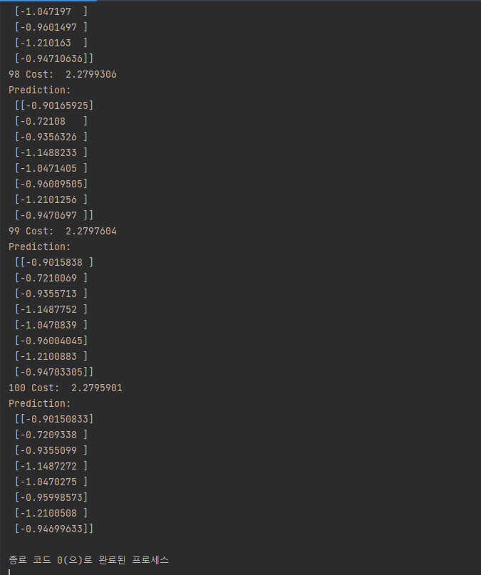

xy = MinMaxScaler(xy) 을 주게 되면 제일 작은값을 0 제일 큰값을 1로 줘서 그 사이를 값에 따라서 노말라이즈를 한다

ML lab 07-2: Meet MNIST Dataset

MNIST Dataset

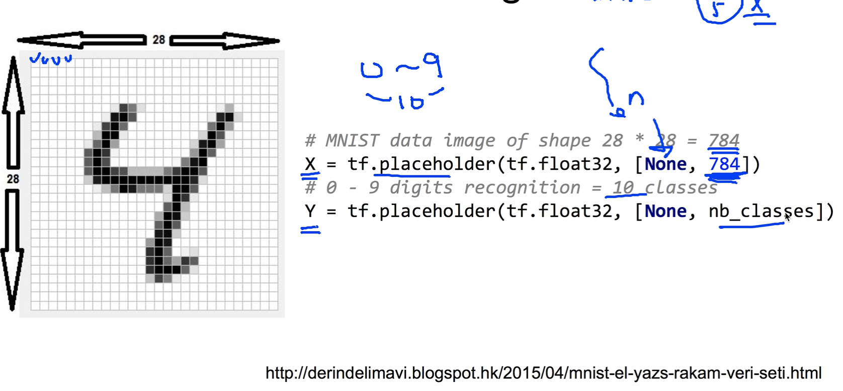
28x28x1 image

MNIST Dataset(code)

import tensorflow.compat.v1 as tf
import matplotlib.pyplot as plt
import numpy as np
import random

tf.disable_v2_behavior()

mnist = tf.keras.datasets.mnist
(x_train, y_train), (x_test, y_test) = mnist.load_data()

print(len(x_train), len(y_train), x_train.shape, y_train.shape)
print(len(x_test), len(y_test), x_test.shape, y_test.shape)

x_train, x_test = x_train / 255.0, x_test / 255.0  # Feature scaling 적용

nb_classes = 10;

x_train_new = x_train.reshape(len(x_train), 784)  # 60000 * 784 배열로 변경 - 한행당 이미지 하나
y_train_new = np.zeros((len(y_train), nb_classes))  # 60000 * 10 배열 생성
for i in range(len(y_train_new)):
    y_train_new[i, y_train[i]] = 1  # one-hot encoding

x_test_new = x_test.reshape(len(x_test), 784)  # 60000 * 784 배열로 변경 - 한행당 이미지 하나
y_test_new = np.zeros((len(y_test), nb_classes))  # 60000 * 10 배열 생성
for i in range(len(y_test_new)):
    y_test_new[i, y_test[i]] = 1  # one-hot encoding

# MNIST data image of shape 28 * 28 = 784
X = tf.placeholder(tf.float32, [None, 784])
# 0 - 9 digits recognition = 10 classes
Y = tf.placeholder(tf.float32, [None, nb_classes])  # 6만개의 학습에 대한 10개의 가설 결과

W = tf.Variable(tf.random_normal([784, nb_classes]))  # 가설이 10개이고 가설별로 784개의 weigh을 가짐, 즉 7840개의 w
b = tf.Variable(tf.random_normal([nb_classes]))  # 가설이 10개니 가설의 b도 10

# Hypothesis (using softmax)
hypothesis = tf.nn.softmax(tf.matmul(X, W) + b)  # 60000 x 10 행렬 - 행별로 열의 값을 확율로 바꿈

# cross entropy
cost = tf.reduce_mean(-tf.reduce_sum(Y * tf.log(hypothesis), axis=1))
optimizer = tf.train.GradientDescentOptimizer(learning_rate=0.1).minimize(cost)

# Test model
is_correct = tf.equal(tf.arg_max(hypothesis, 1), tf.arg_max(Y, 1))
# Calculate accuracy
accuracy = tf.reduce_mean(tf.cast(is_correct, tf.float32))

# parameters
training_epochs = 15  # traing을 몇번 돌릴것인지
batch_size = 100  # 한번에 몇건씩 읽은것인지
total_batch = int(len(x_train_new) / batch_size)

with tf.Session() as sess:
    # Initialize TensorFlow variables
    sess.run(tf.global_variables_initializer())
    # Training cycle
    for epoch in range(training_epochs):
        avg_cost = 0

        for i in range(total_batch):
            # print (epoch,batch_size )
            batch_xs = x_train_new[(epoch * batch_size):(epoch + 1) * batch_size]
            batch_ys = y_train_new[(epoch * batch_size):(epoch + 1) * batch_size]

            _, cost_val = sess.run([optimizer, cost], feed_dict={X: batch_xs, Y: batch_ys})
            avg_cost += cost_val / total_batch

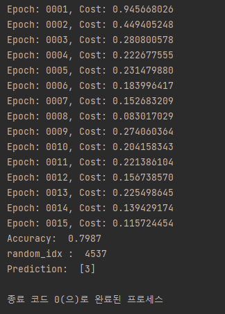
        print("Epoch: {:04d}, Cost: {:.9f}".format(epoch + 1, avg_cost))

    # Test the model using test sets
    print(
        "Accuracy: ",
        accuracy.eval(
            session=sess, feed_dict={X: x_test_new, Y: y_test_new}
        ),
    )

    # Get one and predict
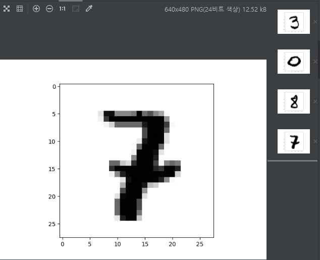
    random_idx = random.randrange(1, 10000)
    print("random_idx : ", random_idx)
    print(
        "Prediction: ",
        sess.run(tf.argmax(hypothesis, 1), feed_dict={X: x_test_new[random_idx: random_idx + 1]}),
    )

    plt.imshow(
        x_test_new[random_idx: random_idx + 1].reshape(28, 28),
        cmap="Greys",
        interpolation="nearest",
    )
    plt.show()