✅ 오늘의 목표
- EDA
오늘부터 시작해서 일요일까지 해야 할 일은 EDA를 통해 데이터를 간단히 살펴보고, 어떻게 전처리하면 좋을지 기준을 세워보는 것.
다른 사람들은 어떤지 모르겠는데, 나는 이 단계에서 가장 설레는 것 같다. 어차피 모델링 쪽은 코드 뚝딱뚝딱하면 금방 끝나지만, EDA는 하나하나 다 그 근거를 설정해야 하고, 우리만의 기준을 세우는 과정이 뭐랄까… 데이터분석가답다 라고나 할까?
자, 이제 본격적으로 프로젝트를 시작해보자!
1. 데이터 간단히 살펴보기
1-1. 데이터 정보 요약
먼저, 우리의 데이터 셋은 다음과 같이 생겼다.
merge_df.info()<class 'pandas.core.frame.DataFrame'>
RangeIndex: 119160 entries, 0 to 119159
Data columns (total 24 columns):
# Column Non-Null Count Dtype
--- ------ -------------- -----
0 order_id 119160 non-null object
1 customer_id 119160 non-null object
2 order_status 119160 non-null object
3 order_purchase_timestamp 119160 non-null object
4 order_approved_at 118982 non-null object
5 order_delivered_timestamp 115738 non-null object
6 order_estimated_delivery_date 119160 non-null object
7 customer_zip_code_prefix 119160 non-null int64
8 customer_city 119160 non-null object
9 customer_state 119160 non-null object
10 order_item_id 118325 non-null float64
11 product_id 118325 non-null object
12 seller_id 118325 non-null object
13 price 118325 non-null float64
14 shipping_charges 118325 non-null float64
15 payment_sequential 119157 non-null float64
16 payment_type 119157 non-null object
17 payment_installments 119157 non-null float64
18 payment_value 119157 non-null float64
19 product_category_name 117893 non-null object
20 product_weight_g 118305 non-null float64
21 product_length_cm 118305 non-null float64
22 product_height_cm 118305 non-null float64
23 product_width_cm 118305 non-null float64
dtypes: float64(10), int64(1), object(13)
memory usage: 21.8+ MB- 총 119,160개의 행
- 총 24개의 열
1-2. 결측치 확인
merge_df.isna().sum()order_id 0
customer_id 0
order_status 0
order_purchase_timestamp 0
order_approved_at 178
order_delivered_timestamp 3422
order_estimated_delivery_date 0
customer_zip_code_prefix 0
customer_city 0
customer_state 0
order_item_id 835
product_id 835
seller_id 835
price 835
shipping_charges 835
payment_sequential 3
payment_type 3
payment_installments 3
payment_value 3
product_category_name 1267
product_weight_g 855
product_length_cm 855
product_height_cm 855
product_width_cm 855
dtype: int64- 총 16 개의 열에 결측치가 존재한다.
- 동일한 개수의 결측치를 갖는 열들이 존재하는데, 분석할 때 같이 봐도 좋을 것 같다.
그리고 수치형과 범주형 변수를 나눠서 살펴봤다.
수치형:
order_item_idpriceshipping_chargespayment_sequentialpayment_installmentspayment_valueproduct_weight_g,product_length_cm,product_height_cm,product_width_cm
범주형:
order_statusorder_purchase_timestamp,order_approved_at,order_delivered_timestamp,order_estimated_delivery_date: 나중에 분기별로 혹은 달별로 범주를 나눠 사용하면 좋을듯customer_zip_code_prefix,customer_city,customer_statepayment_typeproduct_category_name
numerical_cols = ['order_item_id', 'price', 'shipping_charges', 'payment_sequential', 'payment_installments', 'payment_value',
                           'product_weight_g', 'product_length_cm', 'product_height_cm', 'product_width_cm']
categorical_cols = ['order_status', 'order_purchase_timestamp', 'order_approved_at', 'order_delivered_timestamp',
                             'order_estimated_delivery_date', 'customer_zip_code_prefix', 'customer_city', 'customer_state',
                             'payment_type', 'product_category_name']
1-3. 수치형 변수에 대한 value_counts
numerical_df = merge_df[numerical_cols]

for col in numerical_df.columns:
    print(numerical_df[col].value_counts().to_frame().join(numerical_df[col].value_counts(normalize=True).to_frame().cumsum()))
print("=" * 50)- 결과:
                count  proportion
order_item_id
1.0            103656    0.876028
2.0             10314    0.963195
3.0              2403    0.983503
4.0               995    0.991912
5.0               473    0.995910
6.0               264    0.998141
7.0                62    0.998665
8.0                37    0.998977
9.0                29    0.999222
10.0               26    0.999442
11.0               17    0.999586
12.0               13    0.999696
13.0                8    0.999763
14.0                7    0.999823
15.0                5    0.999865
16.0                3    0.999890
17.0                3    0.999915
18.0                3    0.999941
19.0                3    0.999966
20.0                3    0.999992
21.0                1    1.000000
==================================================
        count  proportion
price
59.90    2628    0.022210
69.90    2116    0.040093
49.90    2049    0.057410
89.90    1632    0.071202
99.90    1531    0.084141
...       ...         ...
424.90      1    0.999966
234.80      1    0.999975
119.95      1    0.999983
107.94      1    0.999992
213.39      1    1.000000

[5968 rows x 2 columns]
==================================================
                  count  proportion
shipping_charges
15.10              3856    0.032588
7.78               2353    0.052474
14.10              1989    0.069284
11.85              1982    0.086034
18.23              1631    0.099818
...                 ...         ...
39.37                 1    0.999966
49.03                 1    0.999975
40.72                 1    0.999983
48.10                 1    0.999992
36.89                 1    1.000000

[6999 rows x 2 columns]
==================================================
                     count  proportion
payment_sequential
1.0                 114011    0.956813
2.0                   3430    0.985599
3.0                    662    0.991155
4.0                    320    0.993840
5.0                    192    0.995451
6.0                    134    0.996576
7.0                     92    0.997348
8.0                     61    0.997860
9.0                     50    0.998280
10.0                    41    0.998624
11.0                    35    0.998917
12.0                    27    0.999144
13.0                    16    0.999278
14.0                    13    0.999387
15.0                    11    0.999480
16.0                     9    0.999555
18.0                     9    0.999631
17.0                     9    0.999706
19.0                     9    0.999782
21.0                     6    0.999832
20.0                     6    0.999883
22.0                     3    0.999908
25.0                     2    0.999924
26.0                     2    0.999941
23.0                     2    0.999958
24.0                     2    0.999975
27.0                     1    0.999983
29.0                     1    0.999992
28.0                     1    1.000000
==================================================
                      count  proportion
payment_installments
1.0                   59438    0.498821
2.0                   13865    0.615180
3.0                   11883    0.714906
4.0                    8073    0.782656
10.0                   6975    0.841193
5.0                    6102    0.892402
8.0                    5109    0.935279
6.0                    4670    0.974471
7.0                    1857    0.990055
9.0                     747    0.996324
12.0                    166    0.997717
15.0                     94    0.998506
18.0                     38    0.998825
24.0                     34    0.999110
11.0                     26    0.999329
20.0                     21    0.999505
13.0                     18    0.999656
14.0                     16    0.999790
17.0                      8    0.999857
16.0                      7    0.999916
21.0                      5    0.999958
0.0                       3    0.999983
23.0                      1    0.999992
22.0                      1    1.000000
==================================================
               count  proportion
payment_value
50.00            351    0.002946
100.00           302    0.005480
20.00            289    0.007906
77.57            251    0.010012
35.00            167    0.011414
...              ...         ...
202.55             1    0.999966
268.97             1    0.999975
381.76             1    0.999983
202.53             1    0.999992
182.39             1    1.000000

[29077 rows x 2 columns]
==================================================
                  count  proportion
product_weight_g
200.0              7092    0.059947
150.0              5414    0.105710
250.0              4727    0.145666
300.0              4444    0.183230
400.0              3780    0.215181
...                 ...         ...
726.0                 1    0.999966
8575.0                1    0.999975
3598.0                1    0.999983
11025.0               1    0.999992
2676.0                1    1.000000

[2204 rows x 2 columns]
==================================================
                   count  proportion
product_length_cm
16.0               18420    0.155699
20.0               10976    0.248476
30.0                7954    0.315709
17.0                6208    0.368184
18.0                5902    0.418072
...                  ...         ...
83.0                   8    0.999831
96.0                   8    0.999899
94.0                   6    0.999949
9.0                    4    0.999983
8.0                    2    1.000000

[99 rows x 2 columns]
==================================================
                   count  proportion
product_height_cm
10.0               10375    0.087697
20.0                6935    0.146317
15.0                6880    0.204471
12.0                6533    0.259693
11.0                6427    0.314019
...                  ...         ...
98.0                   3    0.999932
92.0                   3    0.999958
94.0                   2    0.999975
97.0                   2    0.999992
89.0                   1    1.000000

[102 rows x 2 columns]
==================================================
                  count  proportion
product_width_cm
20.0              12727    0.107578
11.0              11140    0.201741
15.0               9373    0.280969
16.0               8859    0.355851
30.0               8046    0.423862
...                 ...         ...
103.0                 1    0.999966
97.0                  1    0.999975
104.0                 1    0.999983
98.0                  1    0.999992
86.0                  1    1.000000

[95 rows x 2 columns]
==================================================
1-4. 범주형 변수 value_counts
categorical_df = merge_df[categorical_cols]

for col in categorical_df.columns:
    print(categorical_df[col].value_counts().to_frame().join(categorical_df[col].value_counts(normalize=True).to_frame().cumsum()))
print("=" * 50)- 결과:
               count  proportion
order_status
delivered     115739    0.971291
shipped         1257    0.981840
canceled         752    0.988150
unavailable      653    0.993630
processing       376    0.996786
invoiced         375    0.999933
created            5    0.999975
approved           3    1.000000
==================================================
                          count  proportion
order_purchase_timestamp
8/8/2017 20:26               63    0.000529
9/23/2017 14:56              38    0.000848
8/2/2018 12:06               35    0.001141
8/2/2018 12:05               31    0.001401
4/20/2017 12:45              29    0.001645
...                         ...         ...
8/17/2018 7:44                1    0.999966
12/26/2017 14:16              1    0.999975
7/6/2018 19:14                1    0.999983
10/15/2017 18:32              1    0.999992
3/8/2018 20:57                1    1.000000

[88789 rows x 2 columns]
==================================================
                   count  proportion
order_approved_at
1/10/2018 10:32      121    0.001017
12/1/2017 11:31       94    0.001807
7/24/2018 10:31       88    0.002547
11/7/2017 7:30        87    0.003278
2/27/2018 4:31        82    0.003967
...                  ...         ...
8/23/2017 20:15        1    0.999966
7/3/2017 16:30         1    0.999975
7/28/2018 0:25         1    0.999983
10/7/2016 23:13        1    0.999992
9/14/2017 12:30        1    1.000000

[50462 rows x 2 columns]
==================================================
                           count  proportion
order_delivered_timestamp
8/14/2017 12:46               63    0.000544
10/18/2017 22:35              38    0.000873
3/5/2018 15:22                30    0.001132
6/22/2017 16:04               27    0.001365
2/28/2018 20:09               26    0.001590
...                          ...         ...
1/31/2018 19:16                1    0.999965
11/8/2017 13:42                1    0.999974
6/5/2018 0:44                  1    0.999983
7/27/2018 19:56                1    0.999991
3/16/2018 13:08                1    1.000000

[75649 rows x 2 columns]
==================================================
                               count  proportion
order_estimated_delivery_date
12/20/2017 0:00                  658    0.005522
3/12/2018 0:00                   617    0.010700
3/13/2018 0:00                   616    0.015869
5/29/2018 0:00                   615    0.021031
5/30/2018 0:00                   593    0.026007
...                              ...         ...
11/14/2016 0:00                    1    0.999966
11/7/2016 0:00                     1    0.999975
1/9/2017 0:00                      1    0.999983
10/28/2016 0:00                    1    0.999992
10/27/2016 0:00                    1    1.000000

[459 rows x 2 columns]
==================================================
                          count  proportion
customer_zip_code_prefix
24220                       163    0.001368
22790                       156    0.002677
22793                       155    0.003978
24230                       139    0.005144
22775                       132    0.006252
...                         ...         ...
58086                         1    0.999966
68798                         1    0.999975
55365                         1    0.999983
89086                         1    0.999992
45920                         1    1.000000

[14994 rows x 2 columns]
==================================================
                     count  proportion
customer_city
sao paulo            18864    0.158308
rio de janeiro        8322    0.228147
belo horizonte        3310    0.255925
brasilia              2488    0.276804
curitiba              1827    0.292137
...                    ...         ...
igrapiuna                1    0.999966
nantes                   1    0.999975
carnauba dos dantas      1    0.999983
satiro dias              1    0.999992
nova vicosa              1    1.000000

[4119 rows x 2 columns]
==================================================
                count  proportion
customer_state
SP              50305    0.422163
RJ              15527    0.552467
MG              13826    0.668496
RS               6542    0.723397
PR               6038    0.774068
SC               4355    0.810616
BA               4091    0.844948
DF               2505    0.865970
GO               2461    0.886623
ES               2366    0.906479
PE               1905    0.922466
CE               1567    0.935616
MT               1131    0.945107
PA               1124    0.954540
MA                859    0.961749
MS                850    0.968882
PB                645    0.974295
PI                577    0.979137
RN                574    0.983954
AL                465    0.987857
SE                409    0.991289
TO                340    0.994142
RO                293    0.996601
AM                174    0.998061
AC                 95    0.998859
AP                 84    0.999564
RR                 52    1.000000
==================================================
              count  proportion
payment_type
credit_card   87795    0.736801
wallet        23177    0.931309
voucher        6475    0.985649
debit_card     1707    0.999975
not_defined       3    1.000000
==================================================
                                   count  proportion
product_category_name
toys                               88791    0.753149
health_beauty                       3143    0.779809
bed_bath_table                      2752    0.803152
sports_leisure                      2404    0.823543
computers_accessories               2275    0.842841
...                                  ...         ...
fashion_childrens_clothes              2    0.999966
diapers_and_hygiene                    1    0.999975
home_comfort_2                         1    0.999983
furniture_mattress_and_upholstery      1    0.999992
security_and_services                  1    1.000000

[70 rows x 2 columns]
==================================================
2. 데이터 시각화
📊 데이터 종류별 시각화 방법은 다음과 같이 선정했다:
수치형 시각화 방법:
- 히스토그램 : histplot()
- 커널밀도추정함수 그래프 : kdeplot()
- 박스플롯 : boxplot()
범주형 시각화 방법:
- 카운트플롯 : countplot()
2-1. 수치형 시각화
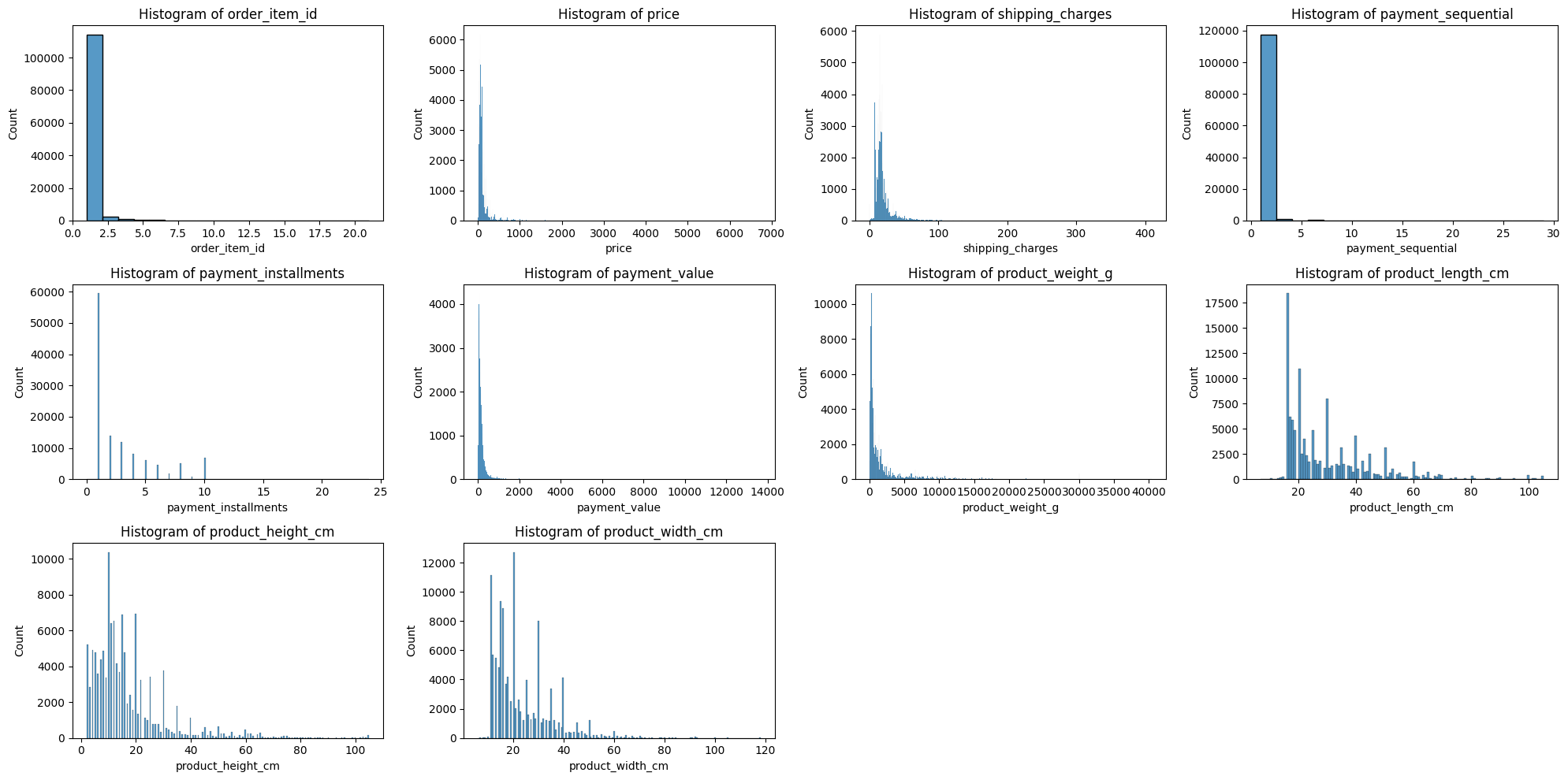
📊 히스토그램
plt.figure(figsize=(20, 10))

for idx, col in enumerate(numerical_cols):
    plt.subplot(3, 4, idx+1)
    ax = sns.histplot(merge_df[col], kde=False)
    plt.title(f'Histogram of {col}')

plt.tight_layout()
plt.show()- 결과:
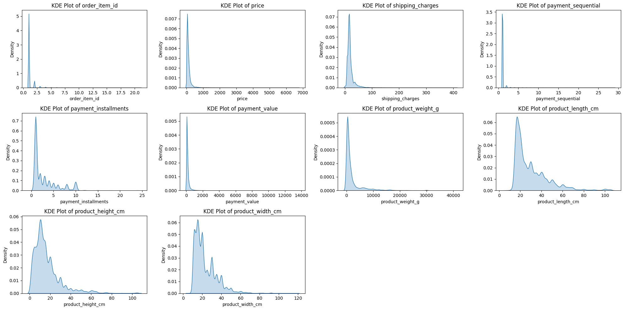
📊 커널밀도추정 그래프
plt.figure(figsize=(20, 10))

for idx, col in enumerate(numerical_cols):
    plt.subplot(3, 4, idx+1)
    ax = sns.kdeplot(merge_df[col], shade=True)
    plt.title(f'KDE Plot of {col}')

plt.tight_layout()
plt.show()- 결과:
📊 박스플롯
plt.figure(figsize=(20, 10))

for idx, col in enumerate(numerical_cols):
    plt.subplot(3, 4, idx+1)
    sns.boxplot(y=merge_df[col])
    plt.title(f'Boxplot of {col}')
    plt.xlabel(col)
    plt.ylabel('Value')

plt.tight_layout()
plt.show()- 결과:
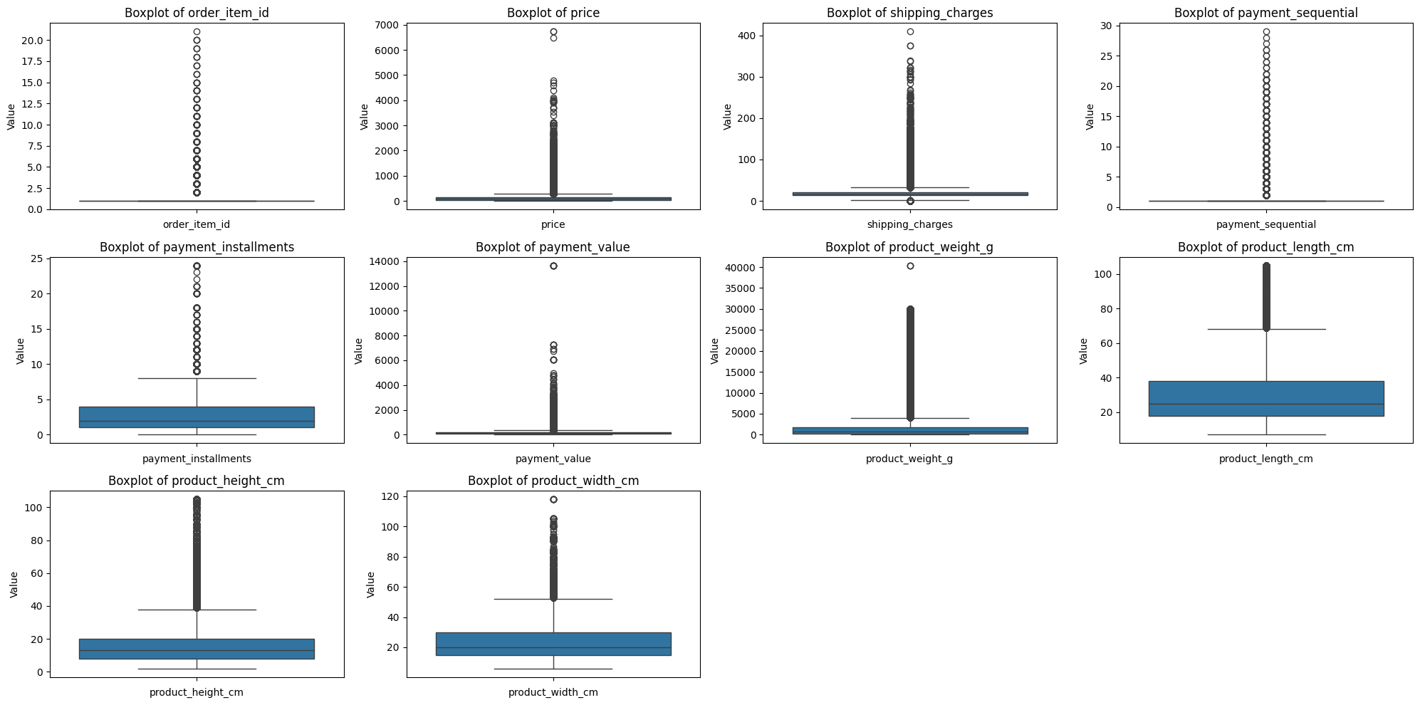
수치형 변수 시각화 해석:
- 시각화 결과 모든 column에서 오른쪽으로 꼬리가 길게 늘어진 현상(right-skewed) 발견.
- 데이터의 표준화가 필요할 거 같다.
- 박스플롯을 살펴봤을 때 이상치가 많아 정제가 필요할 거 같다.
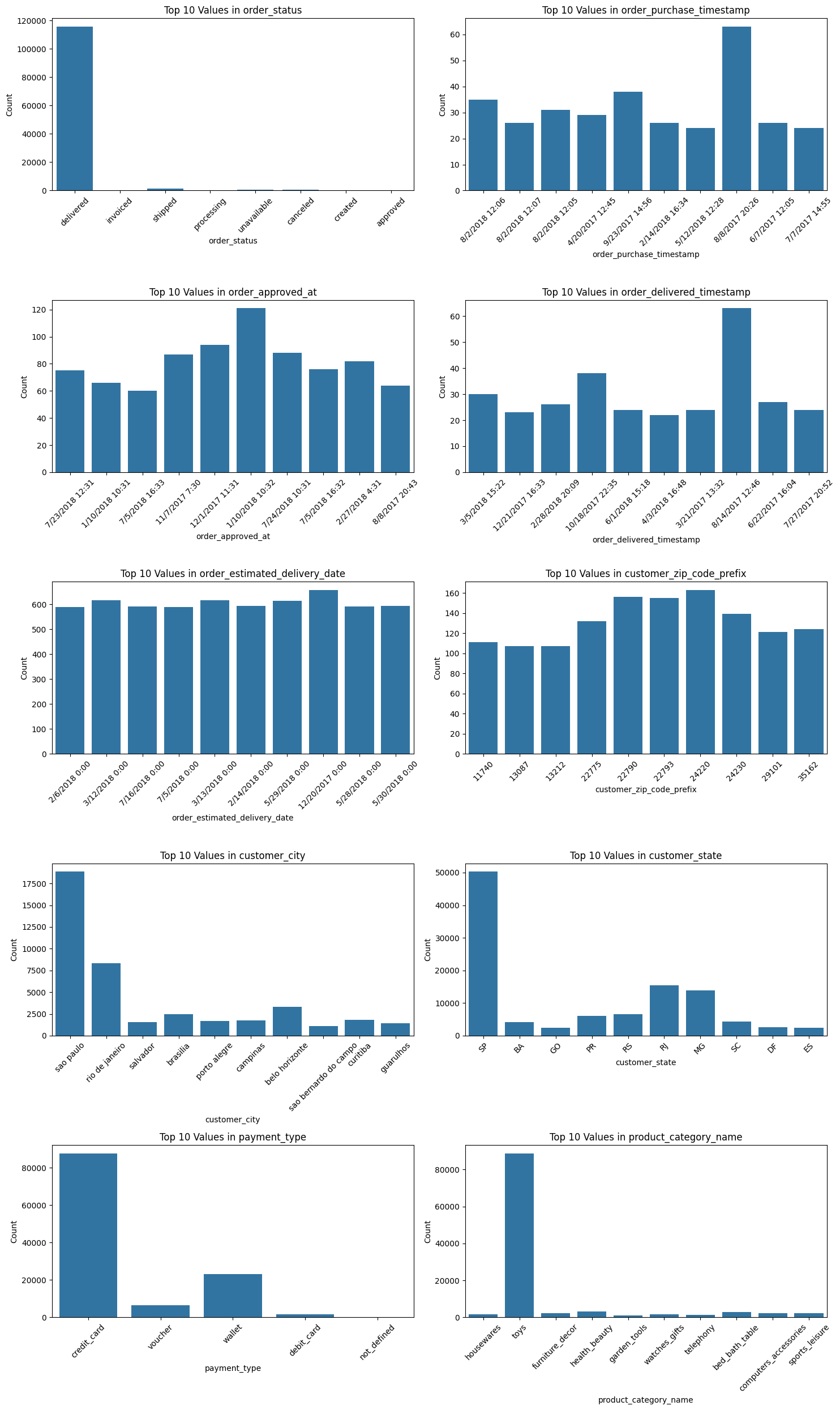
2-2. 범주형 시각화
📊 박스플롯
- 카테고리의 개수가 많아서 제대로 된 결과를 볼 수 없기 때문에 상위 10개 까지의 카테고리만 살펴봤다.
rows = 5
cols = 2

# 플롯 크기 설정
fig, axes = plt.subplots(rows, cols, figsize=(15, 25))

# 모든 플롯을 차지할 수 있도록 축 배열 평탄화
axes = axes.flatten()

# 각 범주형 변수에 대해 상위 10개 값의 countplot 그리기
for i, col in enumerate(categorical_cols):
    top_10_values = merge_df[col].value_counts().nlargest(10).index
    sns.countplot(data=merge_df[merge_df[col].isin(top_10_values)], x=col, ax=axes[i])
    axes[i].set_title(f'Top 10 Values in {col}')
    axes[i].set_ylabel('Count')
    axes[i].set_xlabel(col)
    axes[i].tick_params(axis='x', rotation=45)

# 레이아웃 조정
plt.tight_layout()
plt.show()- 결과:
오늘의 소감
SQLD 자격증 시험
- 난이도가 생각보다는 쉬웠던 것 같다. 프로젝트에 시간을 많이 쓰느라 공부를 많이 못 했는데, 한두 번 정도만 더 훑어봤어도 자신 있게 합격을 기대했을 것 같은데… 선택과 집중을 제대로 하지 못했던 것 같아 아쉬움이 남는다.
프로젝트
- subplot을 사용해 플롯의 크기를 설정해 여러 개의 그래프를 이쁘게 출력하는 방법을 알게 됐다.
- fig: 프레임 크기
- ax: 그래프를 그릴 캔버스
- 변수의 형태별 시각화 방법을 고려해 본 것도 좋은 시도였던 것 같다.
- 수치형과 범주형 변수를 나누는 부분이 아직 헷갈리는 것 같다. 조금 더 연습해 볼 필요가 있다고 느꼈다.
- Velog에는 왜 토글이 없을까...
ㅂㄷㅂㄷ
내일 할 일
- EDA 결과를 토대로 데이터 전처리

데이터분석 공부 일기~!