✅ 오늘의 목표
- 데이터 전처리
오늘은 팀원들 각자 EDA 및 전처리 기준에 대해 고민했던 것들을 논의하며 최종 결론을 내는 날.
1. 결측치 처리
결측치가 있었던 열은 다음과 같았다:
merge_df[missing_columns].isna().sum()- 결과:
order_approved_at             178
order_delivered_timestamp    3422
order_item_id                 835
product_id                    835
seller_id                     835
price                         835
shipping_charges              835
payment_sequential              3
payment_type                    3
payment_installments            3
payment_value                   3
product_category_name        1267
product_weight_g              855
product_length_cm             855
product_height_cm             855
product_width_cm              855
dtype: int64
지금부터 각 열에 대한 기준을 세워보도록 하자!
1-1. order_approved_at
order_approved_at은 주문이 승인된 시간으로 order_status 컬럼과 연관이 있을 것 같아 함께 살펴봤다.
# 'order_approved_at' 컬럼에서 결측치가 포함된 행만 추출
missing_rows = merge_df[merge_df['order_approved_at'].isna()]

# 'order_status' 컬럼의 value_counts
order_status_counts = missing_rows['order_status'].value_counts()
print("Order Status Counts:")
print(order_status_counts)- 결과:
Order Status Counts:
order_status
canceled     158
delivered     15
created        5
Name: count, dtype: int64
- canceled 인 경우 당연하게도 주문이 승인이 되지 않기 때문에 결측치가 발생.
- delivered 됐는데 승인이 되지 않은 경우가 15건 있는데, 시스템 오류로 발생한 결측치로 보는 것이 타당하다고 생각.
- created 또한 마찬가지로 시스템 오류로 보는 것이 합당할 듯.
결론: order_approved_at 의 결측치는 178개인데, 전체 데이터에 비하면 그 비율이 너무 작기에 그것을 알아내는 비용이 이유를 알아냈을 때 얻을 수 있는 이득보다 더 클 것이라 생각되어 행을 제거하면 어떨까?
1-2. order_delivered_timestamp
order_delivered_timestamp는 고객 위치에 배송이 완료된 시점의 시간이다. 이 또한 order_status와 함께 봤는데
# 'order_approved_at' 컬럼에서 결측치가 포함된 행만 추출
missing_rows = merge_df[merge_df['order_delivered_timestamp'].isna()]

# 'order_status' 컬럼의 value_counts
order_status_counts = missing_rows['order_status'].value_counts()
print("Order Status Counts:")
print(order_status_counts)- 결과:
Order Status Counts:
order_status
shipped        1257
canceled        745
unavailable     653
processing      376
invoiced        375
delivered         8
created           5
approved          3
Name: count, dtype: int64
- order_status가 delivered 가 아닌 경우 당연하게도 배송된 시점의 타임스탬프는 비어있어야한다. 문제는 delivered 됐는데도 타임스탬프가 비어있는 경우이다.
-
하지만 그 개수가 8개로 행 제거.
-
그리고 나머지 status에 대해서 결측치가 있는 부분은 전자상거래 도메인에 대한 이해가 필요할거 같다.
결론: delivered를 제외한 나머지 상태에서는 아직 도착하지 않았으니 비어있는게 당연하다. 그리고 결측치 개수가 3,422개로 전체 데이터와 비교하면 약 3%정도 된다. 따라서 비어있는 부분은 그대로 두고 나머지 데이터들에 대해서만 분석을 진행해도 되지 않을까?
-
1-3. order_item_id ~ shipping_charges
- order_item_id, product_id, seller_id, price, shipping_charges
위의 컬럼들은 결측치가 모두 835개로 동일했는데, 서로 관계가 있을 것이라 생각하여 order_status와 함께 봤다.
# 체크할 컬럼들 정의
columns_to_check = ['order_item_id', 'product_id', 'seller_id', 'price', 'shipping_charges']

# 각 컬럼에 대해 결측치가 포함된 행들의 'order_status'에 대한 value_counts 계산
for column in columns_to_check:
    # 각 컬럼에 대해 결측치가 있는 행만 필터링
    missing_rows = merge_df[merge_df[column].isna()]

    # 해당 행들의 'order_status' value_counts 계산
    order_status_counts = missing_rows['order_status'].value_counts()

    # 결과 출력
    print(f"Order Status Value Counts for Rows with Missing '{column}':")
    print(order_status_counts)
print("-" * 50) # 구분선 출력- 결과:
Order Status Value Counts for Rows with Missing 'order_item_id':
order_status
unavailable    646
canceled       181
created          5
invoiced         2
shipped          1
Name: count, dtype: int64
--------------------------------------------------
Order Status Value Counts for Rows with Missing 'product_id':
order_status
unavailable    646
canceled       181
created          5
invoiced         2
shipped          1
Name: count, dtype: int64
--------------------------------------------------
Order Status Value Counts for Rows with Missing 'seller_id':
order_status
unavailable    646
canceled       181
created          5
invoiced         2
shipped          1
Name: count, dtype: int64
--------------------------------------------------
Order Status Value Counts for Rows with Missing 'price':
order_status
unavailable    646
canceled       181
created          5
invoiced         2
shipped          1
Name: count, dtype: int64
--------------------------------------------------
Order Status Value Counts for Rows with Missing 'shipping_charges':
order_status
unavailable    646
canceled       181
created          5
invoiced         2
shipped          1
Name: count, dtype: int64
--------------------------------------------------
-
결과에서도 알 수 있지만, 역시 columns_to_check에 해당하는 모든 컬럼들은 order_status의 영향을 받고 있었다.
-
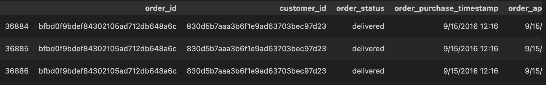
그 중에서도 총 835개 중 646개가
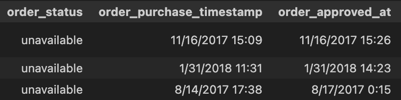
unavailable에 속했다.- unavailable에 속할 경우를 아래와 같이 살펴보면 order_purchase_timestamp, order_approved_at 에는 값이 있는 것으로 보아 판매자 측에서 재고 부족 등의 문제로 취소를 한 경우에 해당한다고 생각.
merge_df[merge_df['order_status'] == 'unavailable'].head(3)- 결과:
- 결과:
- unavailable에 속할 경우를 아래와 같이 살펴보면 order_purchase_timestamp, order_approved_at 에는 값이 있는 것으로 보아 판매자 측에서 재고 부족 등의 문제로 취소를 한 경우에 해당한다고 생각.
-
canceled도 살펴봤을 때 order_purchase_timestamp, order_approved_at에 값이 있는 것으로 보아 본인이 취소한 경우에 속할 것이다.```python merge_df[merge_df['order_status'] == 'canceled'].head(3) ```- 결과:
결론: 이러한 결과들로 살펴봤을 때 본 프로젝트에서는 유효한 주문에 대해서만 분석을 진행하기 위해 835개의 행을 모두 제거하는 것이 좋지 않을까 생각
- 결과:
-
1-4. payment_sequential ~ payment_value
- payment_sequential, payment_type, payment_installments, payment_value
위의 컬럼들은 결측치들이 모두 3개로 동일했기에 함께 살펴봤는데, 3개의 행이 완전히 동일했기에 행을 제거하기로 결정.
columns_to_check2 = ['payment_sequential', 'payment_type', 'payment_installments', 'payment_value']

merge_df[merge_df[columns_to_check2].isna().any(axis=1)]
- 결과:

1-5. product_category_name
product_category_name에서 결측치를 포함하는 데이터의 product_id를 리스트로 뽑고, 이 product_id 들에 대한 다른 행의 product_category_name 중 결측치가 아닌 것을 찾아 제품 카테고리를 역추적할 수 있지 않을까?
# product_category_name이 결측치인 행의 product_id 추출

product_ids = merge_df[merge_df['product_category_name'].isna()]['product_id'].tolist()
product_ids
# product_ids 리스트에 있는 product_id들 중에서, product_category_name이 결측치가 아닌 행들을 필터링
filtered_df = merge_df[merge_df['product_id'].isin(product_ids) & merge_df['product_category_name'].notna()]
filtered_df
- 결과:
- 확인 결과 없었다.
결론: 해당 product_category_name은 아마 이제 더이상 판매하지 않는 제품들인거 같으므로, 삭제하는 것이 마땅하다고 생각.
1-6. product_weight_g ~ product_width_cm
- product_weight_g, product_length_cm, product_height_cm, product_width_cm
- 해당 컬럼들에 대해서는 전체 데이터 개수 대비 0.71%로 매우 작지만, 극단값의 영향을 줄이기 위해 중앙값으로 대체
최종 결측치 처리하는 코드
# 각 컬럼의 중앙값으로 결측치를 채우기 [product_weight_g, product_length_cm, product_height_cm, product_width_cm]
merge_df['product_weight_g'].fillna(merge_df['product_weight_g'].median(), inplace=True)
merge_df['product_length_cm'].fillna(merge_df['product_length_cm'].median(), inplace=True)
merge_df['product_height_cm'].fillna(merge_df['product_height_cm'].median(), inplace=True)
merge_df['product_width_cm'].fillna(merge_df['product_width_cm'].median(), inplace=True)

# 결측치를 제거할 열 목록
columns_to_drop_null= [
    'order_approved_at',
    'order_item_id',
    'product_id',
    'seller_id',
    'price',
    'shipping_charges',
    'payment_sequential',
    'payment_type',
    'payment_installments',
    'payment_value',
    'product_category_name'
]

# 지정된 열들에서 결측치가 있는 행을 제거
merge_df = merge_df.dropna(subset=columns_to_drop_null)

# 분석 프로젝트에 필요 없다고 판단한 컬럼 제거
columns_to_drop = ['payment_sequential']
merge_df = merge_df.drop(columns=columns_to_drop)

merge_df.isna().sum()- 결과:
order_id 0 customer_id 0 order_status 0 order_purchase_timestamp 0 order_approved_at 0 order_delivered_timestamp 2566 order_estimated_delivery_date 0 customer_zip_code_prefix 0 customer_city 0 customer_state 0 order_item_id 0 product_id 0 seller_id 0 price 0 shipping_charges 0 payment_type 0 payment_installments 0 payment_value 0 product_category_name 0 product_weight_g 0 product_length_cm 0 product_height_cm 0 product_width_cm 0 dtype: int64- 그냥 두기로 한 order_delivered_timestamp 외에 결측치 처리가 잘 된 것을 확인할 수 있다.
2. 이상치 처리
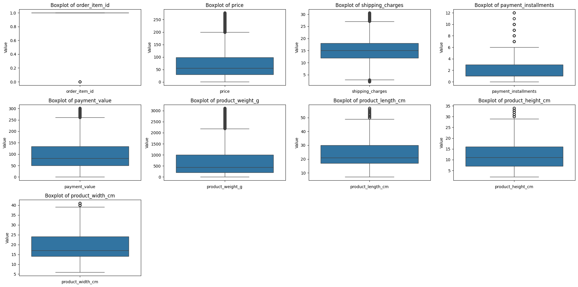
어제 EDA를 통해 살펴봤던 것처럼 모든 수치형 변수들에 이상치가 있는 것으로 확인되어 이상치 처리가 필요한 상황이다.
수치형 변수에 대한 value_counts
numerical_cols = ['order_item_id', 'price', 'shipping_charges', 'payment_installments', 'payment_value',
                           'product_weight_g', 'product_length_cm', 'product_height_cm', 'product_width_cm']
numerical_df = merge_df[numerical_cols]

for col in numerical_df.columns:
    print(numerical_df[col].value_counts().to_frame().join(numerical_df[col].value_counts(normalize=True).to_frame().cumsum()))
print("=" * 50)- 결과:
                count  proportion
order_item_id
1.0            103276    0.876148
2.0             10268    0.963258
3.0              2388    0.983516
4.0               991    0.991924
5.0               471    0.995919
6.0               262    0.998142
7.0                62    0.998668
8.0                36    0.998973
9.0                29    0.999220
10.0               26    0.999440
11.0               17    0.999584
12.0               13    0.999695
13.0                8    0.999762
14.0                7    0.999822
15.0                5    0.999864
16.0                3    0.999890
17.0                3    0.999915
18.0                3    0.999941
19.0                3    0.999966
20.0                3    0.999992
21.0                1    1.000000
==================================================
         count  proportion
price
59.90     2623    0.022252
69.90     2115    0.040195
49.90     2035    0.057459
89.90     1628    0.071270
99.90     1522    0.084182
...        ...         ...
21.94        1    0.999966
869.99       1    0.999975
1019.49      1    0.999983
698.00       1    0.999992
213.39       1    1.000000

[5944 rows x 2 columns]
==================================================
                  count  proportion
shipping_charges
15.10              3838    0.032560
7.78               2340    0.052411
14.10              1976    0.069175
11.85              1966    0.085854
18.23              1627    0.099656
...                 ...         ...
53.02                 1    0.999966
55.84                 1    0.999975
39.37                 1    0.999983
49.03                 1    0.999992
0.62                  1    1.000000

[6992 rows x 2 columns]
==================================================
                      count  proportion
payment_installments
1.0                   58681    0.497824
2.0                   13750    0.614473
3.0                   11778    0.714392
4.0                    8000    0.782261
10.0                   6906    0.840848
5.0                    6040    0.892089
8.0                    5078    0.935169
6.0                    4631    0.974456
7.0                    1841    0.990074
9.0                     736    0.996318
12.0                    164    0.997709
15.0                     94    0.998507
18.0                     38    0.998829
24.0                     34    0.999118
11.0                     25    0.999330
20.0                     21    0.999508
13.0                     18    0.999661
14.0                     16    0.999796
17.0                      7    0.999856
16.0                      7    0.999915
21.0                      5    0.999958
0.0                       3    0.999983
23.0                      1    0.999992
22.0                      1    1.000000
==================================================
               count  proportion
payment_value
50.00            347    0.002944
100.00           300    0.005489
20.00            288    0.007932
77.57            251    0.010062
35.00            164    0.011453
...              ...         ...
526.67             1    0.999966
680.82             1    0.999975
438.81             1    0.999983
561.56             1    0.999992
281.43             1    1.000000

[28878 rows x 2 columns]
==================================================
                  count  proportion
product_weight_g
200.0              7023    0.059580
150.0              5407    0.105451
250.0              4719    0.145485
300.0              4417    0.182957
400.0              3733    0.214626
...                 ...         ...
7034.0                1    0.999966
361.0                 1    0.999975
9167.0                1    0.999983
13805.0               1    0.999992
2676.0                1    1.000000

[2203 rows x 2 columns]
==================================================
                   count  proportion
product_length_cm
16.0               18305    0.155292
20.0               10965    0.248314
30.0                7934    0.315622
17.0                6198    0.368204
18.0                5888    0.418155
...                  ...         ...
83.0                   8    0.999830
96.0                   8    0.999898
94.0                   6    0.999949
9.0                    4    0.999983
8.0                    2    1.000000

[99 rows x 2 columns]
==================================================
                   count  proportion
product_height_cm
10.0               10358    0.087873
20.0                6905    0.146452
15.0                6858    0.204632
12.0                6526    0.259996
11.0                6422    0.314477
...                  ...         ...
98.0                   3    0.999932
92.0                   3    0.999958
94.0                   2    0.999975
97.0                   2    0.999992
89.0                   1    1.000000

[102 rows x 2 columns]
==================================================
                  count  proportion
product_width_cm
20.0              12715    0.107869
11.0              11019    0.201349
15.0               9329    0.280492
16.0               8850    0.355572
30.0               8023    0.423635
...                 ...         ...
103.0                 1    0.999966
97.0                  1    0.999975
104.0                 1    0.999983
98.0                  1    0.999992
86.0                  1    1.000000

[95 rows x 2 columns]
==================================================
2-1. order_item_id
order_item_id에 대한 value_counts를 살펴보면
- 1일 때의 개수가 103,276개로 누적합 약 87.6%를 차지하고 있다.
- 또한 2일 때의 개수가 10,268개로 전체의 약 10%에 해당한다.
결론: 따라서, 1개를 구매한 경우와 2개 이상을 구매한 경우로 이진화하는 방법으로 범주형 변수로 변환하는 것이 나을 것이라 생각
- 1개를 구매한 경우 1, 2개 이상을 구매한 경우를 0으로 변환
- 이진화를 할 경우 불균형 문제를 어느정도 해결할 수 있을 것.
2-2. price
우측으로 꼬리가 긴 right-skewed 분포를 가지기 때문에 모델링에 부정적인 영향을 미칠 수 있다.
결론: 따라서, right-skewed 분포를 가져 극단값이 클러스터링 결과에 큰 영향을 미칠 수 있는 이러한 경우에 사용하면 효과적인 IQR 방법으로 이상치 제거.
2-3. payment_sequential
결론: payment_sequential의 경우 누적합 95%의 값이 1에 집중되어 있다. 따라서, 빈도수가 낮은 값들이 데이터의 왜곡을 초래할 수 있기 때문에, 빈도 기반 필터링을 통해 빈도수가 적은 결제 순서 값을 제거.
(위와 같이 하려고 했으나 회의 결과 분석에 크게 도움이 되지 않을 것이라 판단해 분석에서 제외.)
2-4. payment_installments
결론: payment_installments는 1개월부터 12개월까지 거의 순서대로 나열되어 있으며, 누적합 액 99.8%를 차지한다.
- 따라서, 12개월 그 이상의 할부 개월은 이상치로 보고 필터링.
- 브라질 카드사의 할부 수수료를 보고싶었으나 찾지 못해 국내 카드사를 참고. 3, 6, 9, 12개월 이렇게 3개월마다 수수료가 달라지며 보통 1~12개월까지가 가장 많다고 한다.
2-5. payment_value
결론: price와 연관이 있는 변수로 동일하게 IQR 방법으로 제거.
2-6. shipping_charges
결론: IQR 방법으로 처리
2-7. product_weight_g, product_length_cm, product_height_cm, product_width_cm
결론: 위에서 boxplot을 살펴봤을 때 IQR이 적절해보임
최종 이상치 처리하는 코드
# 변수 이진화 함수
def binarize(df, column_name):
    df[column_name] = df[column_name].apply(lambda x: 1 if x == 1 else 0)
    return df

# IQR 제거 방식
def remove_outliers_iqr(df, column_name):
    Q1 = df[column_name].quantile(0.25)
    Q3 = df[column_name].quantile(0.75)
    IQR = Q3 - Q1

    lower_bound = Q1 - 1.5 * IQR
    upper_bound = Q3 + 1.5 * IQR

    df_cleaned = df[(df[column_name] >= lower_bound) & (df[column_name] <= upper_bound)]

    return df_cleaned

# 빈도수 기반 필터링 함수
def remove_low_frequency_outliers(df, column_name, min_frequency=0.01):
    value_counts = df[column_name].value_counts()
    proportions = value_counts / len(df)

    valid_values = proportions[proportions >= min_frequency].index

    df_cleaned = df[df[column_name].isin(valid_values)]

    return df_cleaned

def remove_outliers_by_threshold(df, column_name, threshold):
    df_cleaned = df[df[column_name] <= threshold]

    return df_cleaned

# order_item_id 1개는 1로, 2개 이상은 0으로 이진화하는 코드
merged_df_cleaned = binarize(merge_df, 'order_item_id')

# price, shipping_charges, payment_value IQR 방법으로 처리
merged_df_cleaned = remove_outliers_iqr(merged_df_cleaned, 'price')
merged_df_cleaned = remove_outliers_iqr(merged_df_cleaned, 'shipping_charges')
merged_df_cleaned = remove_outliers_iqr(merged_df_cleaned, 'payment_value')

# payment_installments 12개월 초과는 필터링
merged_df_cleaned = remove_outliers_by_threshold(merged_df_cleaned, 'payment_installments', 12)

# product_weight_g, product_length_cm, product_height_cm, product_width_cm IQR 방법으로 처리
merged_df_cleaned = remove_outliers_iqr(merged_df_cleaned, 'product_weight_g')
merged_df_cleaned = remove_outliers_iqr(merged_df_cleaned, 'product_length_cm')
merged_df_cleaned = remove_outliers_iqr(merged_df_cleaned, 'product_height_cm')
merged_df_cleaned = remove_outliers_iqr(merged_df_cleaned, 'product_width_cm')
이상치, 결측치 처리 후의 데이터 요약
merged_df_cleaned.to_csv('merged_df_cleaned.csv', index=False)
merged_df_cleaned.info()- 결과:
<class 'pandas.core.frame.DataFrame'>
Index: 77871 entries, 0 to 119159
Data columns (total 23 columns):
 #   Column                         Non-Null Count  Dtype
---  ------                         --------------  -----
 0   order_id                       77871 non-null  object
 1   customer_id                    77871 non-null  object
 2   order_status                   77871 non-null  object
 3   order_purchase_timestamp       77871 non-null  object
 4   order_approved_at              77871 non-null  object
 5   order_delivered_timestamp      76297 non-null  object
 6   order_estimated_delivery_date  77871 non-null  object
 7   customer_zip_code_prefix       77871 non-null  int64
 8   customer_city                  77871 non-null  object
 9   customer_state                 77871 non-null  object
 10  order_item_id                  77871 non-null  int64
 11  product_id                     77871 non-null  object
 12  seller_id                      77871 non-null  object
 13  price                          77871 non-null  float64
 14  shipping_charges               77871 non-null  float64
 15  payment_type                   77871 non-null  object
 16  payment_installments           77871 non-null  float64
 17  payment_value                  77871 non-null  float64
 18  product_category_name          77871 non-null  object
 19  product_weight_g               77871 non-null  float64
 20  product_length_cm              77871 non-null  float64
 21  product_height_cm              77871 non-null  float64
 22  product_width_cm               77871 non-null  float64
dtypes: float64(8), int64(2), object(13)
memory usage: 14.3+ MB
- 수치형 변수
- 결과:

- 결과:
- 처리 전보다 훨씬 괜찮아진 것을 확인 가능.
회의 결과
오늘의 회의하면서 각자 EDA 및 이상치 처리했던 것들 공유하는 시간을 가졌는데, 감사하게도 내가 한 방식이 가장 좋은 것 같다고 해주셔서 데이터 전처리에 내 방법을 사용하기로 했다.
내일 할 일
결측치, 이상치 처리에 이어 변수 스케일링 하기.