
핸즈온 머신러닝+캐글 코드리뷰 스터디를 시작했다.
앞으로 핸즈온 머신러닝 정리와 캐글 코드 리뷰를 기록해보려 한다.
개인적으로 머신러닝을 할 때 고민되는 부분 중 하나가 '어떤 피쳐를 골라야 하나' 라고 생각한다.
대부분의 경우 '유의미해보이는' (a.k.a 뇌피셜) 피쳐들만을 골랐던 것 같다. 하지만 사람의 판단만으로는 오류를 범할 수 있기 때문에, 더 똑똑하게 feature selection을 할 수 있는 방법들이 존재한다.
이번주 범위인 1, 2장은 다소 광범위해서 그 중 Feature Selection에 관한 이론과 캐글 노트북을 리뷰해보도록 하겠다.
Feature Selection이 뭐냐면
모델 학습에 필요한 피쳐들을 선별하는 작업을 의미한다.
피쳐가 너무 많으면 오버피팅의 위험이 있기 때문에 적절한 피쳐를 사용하는 것이 중요하다.
이름이 유사한 Feature Extraction은 차원축소 등의 방법을 사용해서 새로운 피쳐를 도출하는 것이다.
정리하자면, feature selection은 기존에 있는 피쳐들 중 고르는 방법('select')이고, feature extraction은 기존의 것들로부터 새로운 피쳐를 추출하는 방법('extract')이다.
1. Wrapper method

wrapper method는 예측 모델을 사용해서 피쳐의 부분집합을 만들어 시행하면서 최적화된 집합을 찾는 방법인데, 부분집합을 모두 살펴보기 때문에 많은 시간과 비용이 소요된다.
또한 cross-validation으로 테스트할 셋을 따로 두어야 한다고 한다.
- RFE recursive feature elimination: SVM을 사용하여 재귀적으로 제거하는 방법
- SFS: sequential feature selection: greedy algorithm 사용하여 빈 부분 집합에 피쳐를 하나씩 추가하는 방법
등등
2. Filter method

통계적 측정 방법을 사용하여 피쳐들의 상관관계를 알아내는 방법이다.
도움이 되지 않는 피쳐들은 걸러내는 ('filter') 방식이다.
- information gain
- 카이제곱 검정
- t 검정
- 상관계수
3. Embedded method

Embedded는 wrapper와 filter 결합한 방법인데, 어떤 알고리즘의 경우 모델 내부에서 피쳐를 결정하기도 한다.
- Lasso (L1) regularization
- Ridge (L2) regularization
- Decision Tree 기반 모델
📘 Kaggle
data import & stratified sampling
import pandas as pd
import numpy as np
import gc
import warnings
warnings.filterwarnings("ignore")
application_train = pd.read_csv('../input/application_train.csv')
#Stratified Sampling
application_sample1 = application_train.loc[application_train.TARGET==1].sample(frac=0.1, replace=False)
print('label 1 sample size:', str(application_sample1.shape[0]))
application_sample0 = application_train.loc[application_train.TARGET==0].sample(frac=0.1, replace=False)
print('label 0 sample size:', str(application_sample0.shape[0]))
application = pd.concat([application_sample1, application_sample0], axis=0).sort_values('SK_ID_CURR')label 1 sample size: 2482
label 0 sample size: 28269
결측치 제거까지 해준 결과 (30751, 225)의 크기를 가진 데이터임을 확인했다.
Feature Selection
우리의 목표는 226개의 피쳐에서 100개만을 고르는 것이다.
- xxx_support: 이 피쳐를 선택했는지 아닌지 알려주는 리스트
- xxx_feature: xxx_list에서 상관계수가 높았던 상위 100개의 피쳐를 X에서 인덱스로 찾은 후 xxx_feature 리스트로 저장
1. Wrapper Method
RFE는 점점 피쳐 부분 집합의 개수를 줄여가면서 재귀적으로 피쳐를 찾는 것이 목적이다.
모델이 처음의 피쳐 집합으로 학습을 한 후 중요도 계산한 후, 중요도가 덜 한 피쳐를 제거하고 반복한다.
from sklearn.feature_selection import RFE
from sklearn.linear_model import LogisticRegression
rfe_selector = RFE(estimator=LogisticRegression(), n_features_to_select=100, step=10, verbose=5)
rfe_selector.fit(X_norm, y)
rfe_support = rfe_selector.get_support()
rfe_feature = X.loc[:,rfe_support].columns.tolist()
print(str(len(rfe_feature)), 'selected features')100 selected features
2. Filter Method
2.1. Pearson Correlation
# 피어슨 상관계수는 따로 support 와 feature 를 반환하는 함수가 없기 때문에 직접 만들어주었음.
def cor_selector(X, y):
    cor_list = []
    # calculate the correlation with y for each feature
    for i in X.columns.tolist():
        cor = np.corrcoef(X[i], y)[0, 1]
        cor_list.append(cor)
    # replace NaN with 0
    cor_list = [0 if np.isnan(i) else i for i in cor_list]
    # feature name
    cor_feature = X.iloc[:,np.argsort(np.abs(cor_list))[-100:]].columns.tolist()
    # feature selection? 0 for not select, 1 for select
    cor_support = [True if i in cor_feature else False for i in feature_name]
return cor_support, cor_featurecor_support, cor_feature = cor_selector(X, y)
print(str(len(cor_feature)), 'selected features')100 selected features
2.2. Chi-2
카이제곱은 정규 분포에 적용해야 하기 때문에 MinMaxScaler 로 정규화를 해주어야 한다.
from sklearn.feature_selection import SelectKBest
from sklearn.feature_selection import chi2
from sklearn.preprocessing import MinMaxScaler
X_norm = MinMaxScaler().fit_transform(X)
chi_selector = SelectKBest(chi2, k=100)
chi_selector.fit(X_norm, y)
SelectKBest(k=100, score_func=<function chi2 at 0x7fcb09a7ac80>)
chi_support = chi_selector.get_support()
chi_feature = X.loc[:,chi_support].columns.tolist()
print(str(len(chi_feature)), 'selected features')
100 selected features
SelectKBest 모듈은 다음과 같은 목적에서 해당 모델을 쓸 수 있다;
- For regression: f_regression, mutual_info_regression
- For classification: chi2, f_classif, mutual_info_classif
3. Embedded Method
임베드 기법은 sklearn 에서 SelectFromModel 이라는 모듈을 쓰는데 이름에서 알 수 있듯 모델 내에서 바로 피쳐를 선택한다.
이 코드에서는 L1, 랜덤포레스트, LGBM 세 개의 모델을 사용했다.
3.1. L1
from sklearn.feature_selection import SelectFromModel
from sklearn.linear_model import LogisticRegression

embeded_lr_selector = SelectFromModel(LogisticRegression(penalty="l1"), '1.25*median')
embeded_lr_selector.fit(X_norm, y)
SelectFromModel(estimator=LogisticRegression(C=1.0, class_weight=None, dual=False, fit_intercept=True,
intercept_scaling=1, max_iter=100, multi_class='ovr', n_jobs=1,
penalty='l1', random_state=None, solver='liblinear', tol=0.0001,
verbose=0, warm_start=False),
norm_order=1, prefit=False, threshold='1.25*median')
embeded_lr_support = embeded_lr_selector.get_support()
embeded_lr_feature = X.loc[:,embeded_lr_support].columns.tolist()
print(str(len(embeded_lr_feature)), 'selected features')
108 selected features
3.2. Random Forest
from sklearn.feature_selection import SelectFromModel
from sklearn.ensemble import RandomForestClassifier

embeded_rf_selector = SelectFromModel(RandomForestClassifier(n_estimators=100), threshold='1.25*median')
embeded_rf_selector.fit(X, y)
SelectFromModel(estimator=RandomForestClassifier(bootstrap=True, class_weight=None, criterion='gini',
max_depth=None, max_features='auto', max_leaf_nodes=None,
min_impurity_decrease=0.0, min_impurity_split=None,
min_samples_leaf=1, min_samples_split=2,
min_weight_fraction_leaf=0.0, n_estimators=100, n_jobs=1,
oob_score=False, random_state=None, verbose=0,
warm_start=False),
norm_order=1, prefit=False, threshold='1.25*median')
embeded_rf_support = embeded_rf_selector.get_support()
embeded_rf_feature = X.loc[:,embeded_rf_support].columns.tolist()
print(str(len(embeded_rf_feature)), 'selected features')
99 selected features
3.3. LGBM
from sklearn.feature_selection import SelectFromModel
from lightgbm import LGBMClassifier

lgbc=LGBMClassifier(n_estimators=500, learning_rate=0.05, num_leaves=32, colsample_bytree=0.2,
            reg_alpha=3, reg_lambda=1, min_split_gain=0.01, min_child_weight=40)

embeded_lgb_selector = SelectFromModel(lgbc, threshold='1.25*median')
embeded_lgb_selector.fit(X, y)
SelectFromModel(estimator=LGBMClassifier(boosting_type='gbdt', class_weight=None, colsample_bytree=0.2,
learning_rate=0.05, max_depth=-1, min_child_samples=20,
min_child_weight=40, min_split_gain=0.01, n_estimators=500,
n_jobs=-1, num_leaves=32, objective=None, random_state=None,
reg_alpha=3, reg_lambda=1, silent=True, subsample=1.0,
subsample_for_bin=200000, subsample_freq=1),
norm_order=1, prefit=False, threshold='1.25*median')
embeded_lgb_support = embeded_lgb_selector.get_support()
embeded_lgb_feature = X.loc[:,embeded_lgb_support].columns.tolist()
print(str(len(embeded_lgb_feature)), 'selected features')
110 selected features
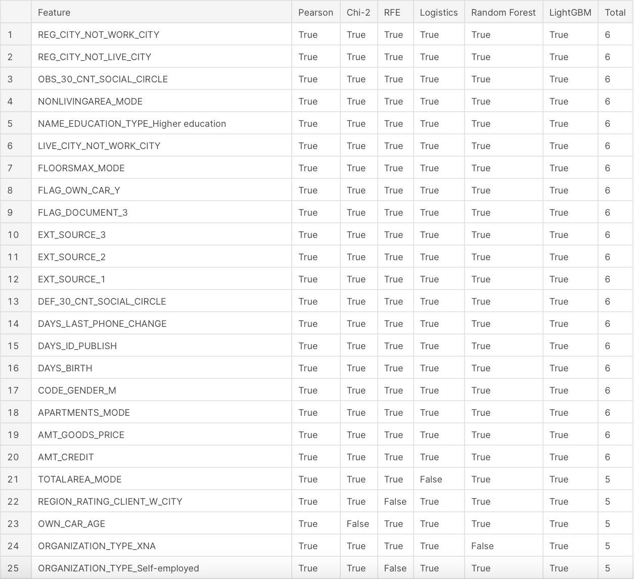
result
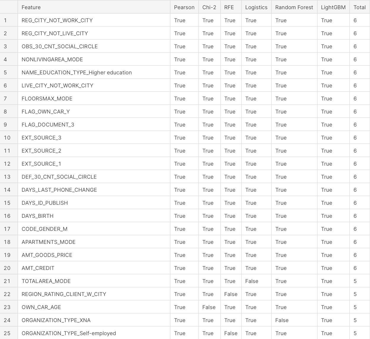
맨 오른쪽 컬럼은 6새의 모델 중 해당 피쳐를 선택한 모델의 개수이다. 상위 20개의 피쳐가 6개의 모델 모두에게 선택된 것으로 보아 대체로 결과가 비슷하다고 해석할 수 있다.
참고자료